Knowledge / Maintenance and reliability
Heat-exchanger tube eddy-current inspection: defect signals, support plates and coverage
Understand what a tube probe actually measures, why support signals can obscure damage, and how skin-depth, complex mixing and coverage calculations must be bounded by calibration evidence.
On this page
An eddy-current tube inspection produces electromagnetic responses, not a direct photograph of the remaining wall. Conductivity, permeability, geometry, probe coupling and discontinuities all affect the recorded signal. The method is powerful when probe configuration and reference standards match the expected damage. It becomes misleading when every phase angle is treated as a universal wall-loss scale or every traversed tube is counted as fully examined.
Begin with the tube material and the expected defect
This article concerns conventional internal eddy-current inspection of non-ferromagnetic heat-exchanger tubes. Material identification is part of the setup: magnetic permeability changes can dominate a conventional response. Methods used for strongly ferromagnetic tubing, such as remote-field techniques or magnetic saturation arrangements, have different physics and qualification needs and should not be substituted by name alone.
An alternating probe field induces currents in the conductive tube. Changes in current paths alter the electrical response of the coils, represented by amplitude and phase or impedance-plane components. A signal is an indication requiring interpretation. Calling it a crack, a pit or a particular percentage of wall loss requires additional evidence from the applicable procedure and reference response.
Standard penetration depth is a scale, not a detection guarantee
Evident describes the reduction of penetration depth as frequency, conductivity or permeability increases. In the ideal homogeneous, semi-infinite planar conductor, standard depth is δ = 1/√(πfμσ), where f is in Hz, μ in H/m and σ in S/m. At depth δ, current-density magnitude is 1/e of its surface value.
An actual thin curved tube with a finite coil is not that ideal geometry. The IAEA manual explicitly limits the planar skin-depth model. It provides a useful parameter for comparing conditions, but it is not a maximum visible depth or a probability of detecting a crack. The practical sensitivity must be demonstrated with the probe and representative reference discontinuities.
Worked frequency comparison: keep the planar assumption visible
Assume a hypothetical nonmagnetic conductor with σ = 1.4 × 10⁶ S/m and μr = 1, using μ0 ≈ 4π × 10⁻⁷ H/m. At 100 kHz, δ = 1.3451 mm; at 400 kHz, δ = 0.67255 mm. Quadrupling frequency halves this ideal depth scale. These assumed material values are not a certificate for a particular installed alloy.
At an illustrative depth of 1.00 mm in the same planar model, J/Jsurface = exp(−x/δ) gives 0.4755 and 0.2261 respectively. Neither number is the amplitude of a real tube-defect signal. A defect perturbs a coupled electromagnetic field, and the receive response depends on geometry and orientation. Do not use these ratios to declare an outer-wall defect detectable or undetectable.
Coil orientation changes which damage is visible
A conventional bobbin arrangement averages response around the circumference and has directional limitations. A discontinuity that substantially interrupts the induced current path can respond differently from one nearly aligned with it. Differential channels emphasize changes between coil locations and can reduce some slowly varying responses; absolute and array channels provide different information.
Eddyfi describes array arrangements intended to address circumferential cracking near support plates and tubesheets, a limitation of conventional bobbin inspection. This explains why probe architecture belongs in the coverage statement. A product’s advertised capability is not evidence that any scan with any option, frequency and calibration has achieved the same detection performance.
Support plates add a real electromagnetic response
A support can change the field even when the adjacent tube is sound. Its material, geometry, clearance and local deposits influence the response. Damage near that support can then appear superimposed on a much larger structural indication. Simply deleting every signal at a known support location would delete the place where relevant fretting or cracking may occur.
Multifrequency mixing is one way to suppress a selected structural response. The IAEA manual describes adjusting amplitude and phase before vector subtraction. Suppression must be checked against representative damage at the support, because the same transformation also acts on the defect response. Retain the original channels so that a clean-looking mixed channel does not become the only evidence.
Worked complex mix: cancel the support and inspect what remains
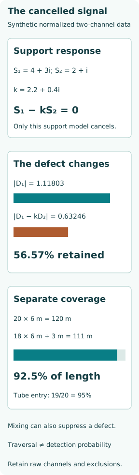
For a synthetic linear example in normalized signal units, let a sound support produce S1 = 4 + 3i and S2 = 2 + i in two channels. Choose k = S1/S2 = 2.2 + 0.4i and form M = Z1 − kZ2. The model cancels that specific support response exactly. This scalar complex coefficient is an illustrative model, not a prescription for a proprietary instrument’s mixing algorithm.
Now suppose a separate defect produces responses D1 = 1 + 0.5i and D2 = 0.2 + 0.1i. After the same mix, D1 − kD2 = 0.6 + 0.2i, magnitude 0.63246. The initial channel-1 defect magnitude was 1.11803, so only 56.57% remains in this comparison. Support cancellation has also reduced defect amplitude. A different support response would leave a residual, and a defect with the cancelled channel ratio could disappear entirely.
Sizing depends on reference morphology, not phase alone
A phase-versus-depth curve is calibrated for particular reference discontinuities, material, tube dimensions and settings. A drilled reference feature and a tight crack do not disturb the same volume or current paths. A curve suitable for one morphology cannot automatically convert another indication into a trustworthy through-wall percentage.
The IAEA discussion distinguishes phase-based and amplitude-based correlations for different tube flaws. A defensible report identifies the sizing method and applicable reference range, rather than presenting a single unexplained wall-loss number. Confirmation with another suitable technique or probe may be needed for ambiguous support-region signals. Acceptance or plugging decisions then apply the equipment’s engineering criteria to the qualified result.
Worked coverage example: entered tubes are not analysed length
Consider 20 planned tubes, each 6 m long, giving 120 m planned length. Suppose 18 are fully traversed and analysable, one is analysable for only 3 m, and one cannot be entered. The entered-tube fraction is 19/20 = 95%, the fully analysed tube fraction 18/20 = 90%, and analysed length is 108 + 3 = 111 m, or 92.5%.
These are three different coverage statements. The simple length example assumes no additional excluded ends, support regions or noisy segments; if such exclusions exist they must also be mapped. Even 100% geometric travel does not prove 100% defect sensitivity, and a percentage of tubes sampled does not by itself establish a probability that the unexamined population is sound.
A reviewable inspection package keeps the missing regions visible
Record the tube map and material, dimensions, probe and cable, frequencies, gain/phase and filters, reference standard, calibration checks, pull speed and data-quality criteria. Link indications and excluded segments to their tube and axial location. Retain the original and mixed channels, the sizing basis and any uncertainty or unclassified indications needed for engineering review.
The useful chain is qualified sensitivity to the expected damage → valid data acquisition → interpreted indications → explicitly mapped coverage → engineering disposition. Skin depth helps explain frequency choice, mixing helps separate signals, and coverage arithmetic describes what was examined. None replaces the other two or turns a clean display into proof of intact tubing.