Vibration spectra and order tracking: diagnosis under changing speed

Define what is being measured

An accelerometer on a bearing housing measures local acceleration along its sensitive axis. It does not directly measure shaft twist, bearing internal force or displacement everywhere in the machine. Mounting stiffness, position, orientation and the transmission path affect the result. A reading from a hand-held probe and a stud-mounted sensor should not be merged without understanding their different response.

Keep amplitude conventions explicit. Acceleration in m/s², velocity in mm/s and displacement in micrometres emphasize different frequency ranges. RMS, peak and peak-to-peak also differ. For a pure sinusoid only, peak equals √2 times RMS. Applying that conversion to an impulsive signal is unjustified. A trend should preserve the quantity, convention, frequency band, mounting and processing settings.

Convert rotational speed to frequency and order

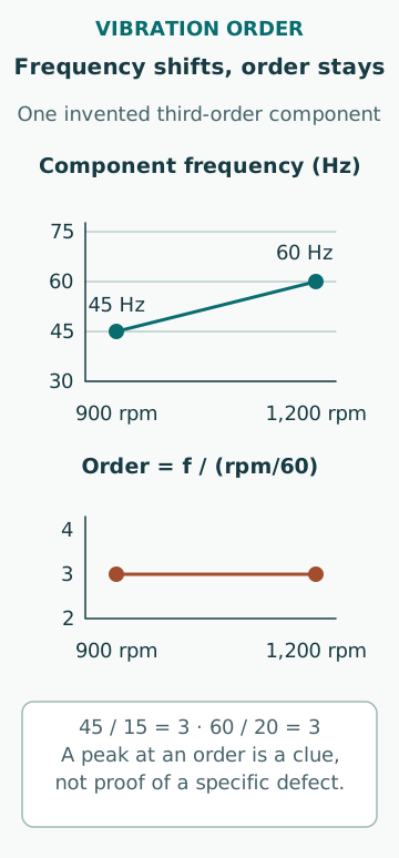
Rotational frequency is n/60 Hz when n is in revolutions per minute. Order is measured frequency divided by that reference rotational frequency. At 900 rpm, shaft frequency is 15 Hz and a 45 Hz component is third order. At 1,200 rpm, the same third-order excitation appears at 60 Hz. A fixed 45 Hz alarm band would then follow a different physical relationship.

For a hypothetical 40-tooth gear on the 900 rpm reference shaft, nominal tooth-mesh frequency is 40 × 15 = 600 Hz, or order 40. Real diagnostic interpretation also needs the gear ratio, reference shaft, sidebands, loading and relevant construction. A peak near a calculated frequency is a hypothesis to test. It does not prove a particular defect, and a gearbox with several shafts needs an unambiguous order reference.

Understand why a changing speed smears a spectrum

A conventional FFT summarizes a finite time record. If a rotating excitation moves from 15 Hz to 20 Hz during that record, its energy spreads over frequencies rather than forming the same narrow line as a steady 15 Hz sinusoid. Shortening the record reduces within-record speed change but worsens frequency spacing. That tradeoff cannot be solved by changing the plot colour or adding decimal places.

NI’s order-analysis explanation describes resampling from equal time increments to equal shaft-angle increments. A component repeating the same number of times per revolution then remains at a stable order. This article uses that general principle, not any proprietary tracking algorithm. Resampling is only as credible as the angular reference and the original signal bandwidth.

Check sampling before interpreting peaks

To represent frequencies below a selected maximum, sampling and analog anti-alias filtering must work together. Frequencies above half the sampling rate can fold into the displayed band. For an illustrative sampling rate of 1,000 samples/s, an unfiltered 700 Hz sinusoid aliases to 300 Hz. Once that ambiguity enters the sampled data, ordinary post-processing cannot determine which physical frequency originally produced it.

Use an acquisition chain with an appropriate usable bandwidth, anti-alias performance and sensor range. Nyquist’s mathematical boundary is not a recommendation to measure right up to the filter edge. Overload and clipping can generate artificial harmonics; a loose sensor or cable motion can create false transients. Review the time waveform and acquisition status as well as the spectrum. A plausible-looking peak can still be an instrumentation artefact.

Distinguish line spacing from resolving power

For a time record of duration T seconds, basic FFT line spacing is 1/T Hz. A 4 s record has 0.25 Hz spacing; a 0.5 s record has 2 Hz spacing. Zero padding draws additional interpolated points but does not create the information of a longer record. Window choice and signal stationarity affect whether two nearby components can actually be separated.

For angle-domain analysis over 40 revolutions, basic order spacing is 1/40 = 0.025 order. At 900 rpm, those 40 revolutions take 2.667 s; at 1,200 rpm they take 2 s. The changing time duration matters when comparing transient processes. Longer records improve nominal order spacing but may combine different loads or operating events. Select the record around the physical question, not merely the smallest available number.

Validate the speed reference and operating comparison

A missing tachometer pulse, an incorrect pulses-per-revolution setting or a reference from the wrong shaft can move every order label. Compare computed speed with a credible independent indication and examine dropouts. NI’s order-tracking overview treats tachometer processing, order magnitude and phase as connected parts of the measurement problem.

Compare the same machine at similar speed, load, valve condition and thermal state. A resonance may amplify a normal excitation over a narrow speed range; load may change hydraulic forces or gear contact. A higher amplitude at a different operating point is not automatically degradation. In a speed sweep, inspect whether a feature follows a constant order, a roughly fixed structural frequency, or a process-related frequency unrelated to shaft speed.

Relate acceleration, velocity and displacement carefully

For a single sinusoidal component, velocity amplitude equals acceleration amplitude divided by 2πf. At f = 25 Hz, an acceleration of 1.0 m/s² RMS corresponds to 0.006366 m/s, or 6.37 mm/s RMS. At 100 Hz the same acceleration corresponds to 1.59 mm/s RMS. Thus an unchanged overall acceleration number does not imply unchanged velocity severity when the frequency content moves.

Integrating a broadband acceleration signal needs attention to low-frequency noise, offsets and filter settings. A derived displacement trace can be dominated by processing artefacts if those are mishandled. Keep the usable integration band and amplitude convention in the report. The calculation above is a dimensional teaching example for a pure sinusoid, not an acceptance threshold or a conversion applicable to every reported overall value.

Do not hide intermittent events with averaging

Averaging can stabilize a spectrum from steady operation, but it can also dilute a short impact or combine two distinct machine states. Keep a record of how many averages were used and whether they were linear, peak-hold or another form. A peak-hold display deliberately retains extremes and should not be compared directly with an ordinary averaged baseline.

For an intermittent complaint, synchronize vibration records with process events such as valve movement, clutch engagement or load transfer. A time waveform can show whether repeated impacts coincide with those events even when the averaged spectrum looks modest. Confirm that clocks are aligned closely enough for the claimed sequence. A useful diagnostic package preserves timing and machine state as well as a visually clean frequency plot.

Turn a spectral observation into a testable diagnosis

Use several observations to distinguish hypotheses: direction, phase, harmonics, sidebands, waveform, temperature, lubricant evidence and maintenance history. A first-order component can occur in more than one fault and in acceptable operation. Bearing characteristic frequencies depend on geometry and kinematics; slip and operating effects can shift them. Avoid a lookup-table diagnosis that ignores the machine’s construction.

Retain raw waveforms and processing settings so another competent analyst can reproduce the result. State what changed, under which conditions, which explanation is supported and which test could disprove it. Applicable machine limits and approved response procedures govern action. Housing-vibration order analysis does not calculate shaft torsional stress or justify entering a barred speed range; those are separate engineering questions.

Sources

• Vibration Analysis and Signal Processing in LabVIEW · NI · Source check date: 2026-10-06
• Performing Order Analysis in LabVIEW with Sound and Vibration Software · NI · Source check date: 2026-10-06