Weibull life data: censoring, mixed populations and maintenance decisions

Choose the observational unit and its clock

Decide whether one record represents a new seal, a complete pump, a bearing after replacement or an operating period following repair. These are different populations. A minor repair does not necessarily return a pump to new condition. Combining successive repaired periods as if they were independent new-component lifetimes silently changes the model.

Choose an exposure clock related to the mechanism. Running hours may suit an operating wear process; starts may better describe cycling damage; calendar time may matter for storage ageing. Record all relevant clocks when possible, but do not switch denominators midway through a fit. A shaft seal operating 400 h during a 1,000 h voyage has 400 running hours and 1,000 calendar hours, not an interchangeable “age.”

Keep right-censored observations

If a bearing is still functioning at 6,000 h when observation ends, its lifetime is greater than 6,000 h. It is right-censored, not a failure at 6,000 h and not an observation to discard. NIST’s censoring chapter distinguishes exact failures, surviving observations and interval information. The survival contribution is valuable evidence even though the eventual failure time is unknown.

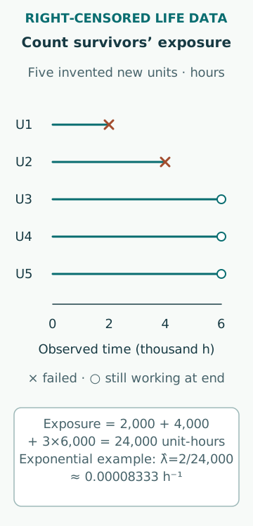
Consider five identical new units: failures occur at 2,000 h and 4,000 h; three survive to 6,000 h. Total observed exposure is 24,000 unit-hours. Under a separate constant-hazard exponential illustration, the maximum-likelihood rate is 2/24,000 = 0.00008333 per hour, whose reciprocal is 12,000 h. Averaging only the two failures gives 3,000 h and answers a different, biased question. The exponential assumption is not a fitted Weibull conclusion.

Read the parameters as model quantities

For a two-parameter Weibull lifetime model, survival is R(t) = exp[−(t/η)^β], where η is the scale in the same time units as t and β is dimensionless shape. At t = η, survival is exp(−1), about 36.8%; η is not generally the mean life; for β = 1 it does equal the mean. The model hazard increases with age for β > 1, stays constant for β = 1 and decreases for β < 1. These statements concern a specified population and clock.

The NIST Weibull reference supplies the distribution relationships. In an original example with assumed β = 2 and η = 10,000 h, survival at 5,000 h is exp(−0.25) = 77.88%. The 10% failure quantile is η[−ln(0.90)]^(1/β) = 3,245.9 h. Calling that quantile a mandatory replacement limit would add a maintenance decision the mathematics does not contain.

Use likelihood terms that match the observation

For a non-informative observation process, an exact failure contributes the density f(t); a right-censored unit contributes survival R(c) at its censoring time c. A failure known only to occur between inspections a and b contributes F(b) − F(a), the probability of failure within that interval. These terms follow from what each observation establishes. The NIST maximum-likelihood overview explains the method’s use with censored data and its small-sample limitations. Replacing every interval by its midpoint falsely presents an uncertain time as exact. If observation ends because degradation is detected, the stopping process needs separate treatment.

For the same assumed Weibull example, the probability of failure between 4,000 h and 5,000 h is exp(−0.16) − exp(−0.25) = 0.07334, or about 7.334% of the original population. Conditional on survival to 4,000 h, the probability is 1 − exp(−0.09) = 8.607%. State which denominator is used. A forecast for units already in service normally needs conditional remaining-life reasoning rather than the unconditional newborn curve.

Question why observation stopped

Study-end censoring is often compatible with ordinary survival analysis. Removal because an operator noticed rising leakage is different: the stopping rule contains information about degradation. Treating such removals as ordinary unrelated censoring can make lifetime estimates too optimistic. Preserve the reason for removal and the condition evidence so an analyst can choose an appropriate method or sensitivity analysis.

Components already old when tracking begins also require attention. If records include only units that survived long enough to enter the database, early failures are absent by design. This delayed entry or left truncation is not repaired by setting every existing unit’s age to zero. Obtain installation dates and entry ages, or state that the selected records cannot support a population lifetime claim.

Avoid mixing mechanisms into a seductive curve

Combine data only when the component design, relevant duty and event definition justify it. Saltwater ingress failures, installation damage and ordinary wear may produce a curved probability plot or a misleading single β. A declining fleet hazard can result from a mixture of weak and robust units; it does not prove that each individual component improves as it ages.

For a mode-specific study, failures from other modes may be represented as competing events, but their independence cannot simply be presumed. Contamination may promote both seal and bearing failure. Stratification can improve interpretability while leaving fewer observations and wider uncertainty. Report that tradeoff instead of hiding it through indiscriminate pooling or selecting the subgroup that produces the most attractive fit.

Distinguish replacement samples from fleet survivors

A workshop’s returned-parts list oversamples failures and excludes most working components. Even perfect failure dates in that list do not define the fleet risk unless the population at risk and its exposure are known. Similarly, a parts purchasing record measures demand for spares, which can include preventive replacement, stock building and warranty exchanges.

Build a reconciliation between installations, removals, failures and end-of-study survivors. Assign each physical unit a stable identity, and distinguish component serial number from equipment tag. If one housing receives three successive bearings, those are three bearing records but one housing. Explain unresolved gaps. A smaller auditable cohort is often more defensible than a large collection of records whose inclusion rules cannot be reconstructed.

Ask what the proposed age replacement would change

An age-replacement calculation compares policies, not just lifetimes. It needs the consequence of an unplanned failure, planned-work duration, repair effectiveness, access constraints and the chance of introducing a defect. Two policies can have similar expected cost but very different tail consequences or operational feasibility.

For example, replacing a part every port call may be impossible when port access does not permit the required isolation. A mathematically attractive 3,000 h age can fall inside a long voyage. Model the actual allowed intervention opportunities and uncertainty in voyage timing. If the result changes sharply when β moves within its uncertainty range, the immediate decision may be to collect better exposure data or use another justified safeguard, rather than treat a fragile optimum as established.

Carry uncertainty into the maintenance decision

A fitted shape greater than one is not sufficient evidence for age replacement. Examine confidence limits, the number and spread of failures, model adequacy and the consequences of intervention. Replacement can introduce defects; useful-life consumption depends on the duty; safety and statutory obligations constrain economic comparisons. A few failures can give highly unstable extrapolations even when software returns many decimal places.

A useful report includes the dataset boundary, exposure clock, failure and censor codes, removal reasons, fitted assumptions, uncertainty and the range of ages supported by observations. Show how the proposed decision changes under plausible parameter and model alternatives. The outcome should be a defensible maintenance choice for the stated population, not a claim that a distribution predicts the exact failure date of a particular shipboard component.

Sources

• Engineering Statistics Handbook: Censoring · NIST · Source check date: 2026-10-06
• Engineering Statistics Handbook: Weibull · NIST · Source check date: 2026-10-06
• Engineering Statistics Handbook: Maximum likelihood estimation · NIST · Source check date: 2026-10-06