Dynamic stability of a dead ship: wind, roll and righting energy

Define the dead-ship condition

Here, “dead ship” identifies a stability problem in which normal propulsion and steering capability are unavailable. It does not mean that the hull stops moving relative to the sea or the ground. Wind, waves and current can still drive drift, yaw and roll, changing exposure as the motion develops.

The subject is therefore different from an electrical restart sequence. Restoring a generator can be essential, but the time-dependent stability response while control is lost needs its own description. A useful model specifies which systems remain effective and which forces act without them. Assuming that every powered stabilizing device remains available would conceal a central consequence of the loss of power.

Separate heel angle from roll motion

Let φ be positive heel toward the wind-driven side, and let φ̇ be the roll rate. Two states with identical φ can have opposite rates: one is moving farther over and the other is returning. Their stored kinetic energies may be equal, but their immediate directions and subsequent interaction with a wave are different.

With effective roll inertia I, kinetic energy is K = ½Iφ̇². The effective inertia represents the modeled ship and associated fluid contribution, not simply displacement multiplied by an arbitrary breadth. An angle record without rate or time history cannot recover this energy. Even a complete instantaneous state does not determine future response until the external forcing and model are specified.

Read the righting-lever curve

Righting moment is mg GZ(φ) under the chosen loading condition and hydrostatic assumptions. Near upright, initial slope can be related to metacentric height, but an energy comparison over a finite angle interval needs the curve over that interval. Extending the initial straight-line approximation far beyond its justified range can change the area and the conclusion.

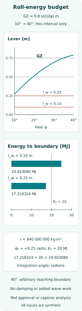
The original case instead declares its entire artificial curve: GZ(φ) = 0.8 sin(2φ) m, used only from 10° to 40°. It is not a measured ship curve and is not extended into an invented downflooding or capsize scenario. Specifying the range is part of specifying the model; the curve outside it contributes nothing to the calculation presented here.

Add wind work to the balance

Represent a steady wind heeling moment as mg l_w, where l_w is a positive constant heeling lever in this exercise. Over a positive roll increment dφ, wind contributes mg l_w dφ of work. The righting moment opposes that increment while GZ remains positive. Their difference determines the increase in the effective potential energy.

A heeling lever is a moment divided by weight, not a wind speed. Converting a measured wind into a moment requires projected area, pressure distribution, lever arms and a stated reference. The chosen levers below are simply inputs. There is no wind-speed limit hidden in either value and no claim that the lever remains constant for an actual vessel at every angle.

Write a bounded roll equation

A one-degree-of-freedom balance can be written Iφ̈ + B(φ̇) + mg[GZ(φ) − l_w] = M_wave(t), with damping moment B opposing motion and wave moment M_wave. This names the physics before simplifying it. Multiplying by φ̇ relates the moment balance to kinetic-energy change and makes the work terms explicit.

For the worked comparison only, set damping and additional wave work to zero over the stated interval. Take m = 10,000,000 kg, g = 9.81 m/s², effective roll radius 8 m, hence I = 640,000,000 kg·m². Start at φ₀ = 10° with φ̇₀ = +0.25 rad/s. The comparison boundary φ_b = 40° is an arbitrary teaching endpoint, not a known opening immersion angle.

Compare the two original energy budgets

The initial kinetic energy is ½ × 640,000,000 × 0.25² = 20.000000 MJ. The righting-lever integral is ∫GZ dφ = 0.4[cos20° − cos80°] = 0.306417777 m·rad. Angle integration uses radians, so the interval is π/6 rad. Integrating numerical degree values without conversion would multiply the result by the wrong angular scale.

For l_w = 0.10 m, the net area is 0.254057900 m·rad and mg times that area is 24.923080 MJ. For l_w = 0.25 m, the area is 0.175518083 m·rad and the energy increment is 17.218324 MJ. The same initial 20 MJ lies between them. GZ exceeds both levers throughout this interval, so the effective potential rises monotonically toward the declared boundary.

Restore the physics omitted by the example

In the conservative comparison, the lower-lever case cannot reach 40° from the specified state, while the higher-lever case has enough kinetic energy to reach it. This is a reachability statement about an artificial interval. It is not a safe/unsafe classification: neither the boundary nor the curve describes a real ship’s failure mechanism.

With damping restored, some energy is dissipated. With wave forcing restored, work may be added or removed according to its phase relative to motion. Free drift changes encounter and wind exposure; coupled motions alter the response. A single energy subtraction no longer replaces the required time history. Nor can an assumed favorable wave phase be carried through an entire irregular sea without evidence.

Respect openings, free surfaces and powered devices

MSC.1/Circ.1627 section 2.2 includes dead-ship vulnerability assessment and explicitly considers downflooding, free surfaces and the effectiveness of anti-roll devices following power loss. These physical conditions can constrain the useful range of a righting-lever analysis. A smooth mathematical GZ curve does not establish that a real opening remains protected throughout the plotted angle range.

For a vessel-specific case, loading and tank states must match the curve, opening locations must be known, and any stabilizing system credited must actually be effective in the assumed condition. A powered device’s normal-service capability is not evidence of its blackout capability. The present example credits no such device and assigns no actual downflooding angle; its endpoint has only an explanatory role.

Relate the lesson to formal assessment

The circular’s prescribed dead-ship assessment is more specific than the simple energy comparison used here. Its defined areas, forcing assumptions and assessment paths must be followed within their intended scope. The calculation above does not implement that procedure. Reusing the word “area” is insufficient to turn a newly invented integral into a completed weather or vulnerability criterion.

ITTC’s 2024 Revision 03 stability-test procedure requires representative model mass properties, restoring characteristics and appropriate damping evidence; dead-ship tests should permit free drift. Those requirements explain why validation needs more than matching one curve. Reproducing an observed roll angle with the wrong inertia or constrained drift can hide compensating errors in a model intended for another loading or environment.

Keep an interpretable stability record

The case record should retain the curve, angle interval, inertia, initial roll rate, wind lever, omitted work terms and integration units together. If only the final energy figures survive, another reader cannot determine which physical question was answered. In this example, the difference between the two budgets comes entirely from changing wind work while keeping the initial state and GZ curve fixed.

For a real ship, current loading, boundaries against flooding, environmental conditions and validated response evidence would be needed before drawing a vessel-specific conclusion. The transferable lesson is that heel, roll rate and energy are connected but distinct descriptions. An unchanged instantaneous angle does not establish unchanged dynamic stability, especially when a loss of control changes which forces and stabilizing systems remain available.

Sources

1. IMO MSC.1/Circ.1627, Interim guidelines on the second generation intact stability criteria. 10 December 2020; original IMO circular reproduced in ClassNK technical-information bundle. Dutch government record lists current version 1. — Circular cover; annex 2.2 (dead ship), especially 2.2.1 and 2.2.2, printed annex pp.10–14 / bundle PDF pp.214–218; annex 2.6 (surf-riding/broaching), especially 2.6.3.4; chapter 3 validation.
2. ITTC 7.5-02-07-04.1, Model Tests on Intact Stability. Revision 03, effective 2024; approved September 2024 — 1; 2; 3.1 and 3.1.1–3.1.4; 3.2–3.5; 4