Dynamic event trees: physical-state branching and feedback

Build a small thermal event tree whose demand times come from energy balance, then track repeated temperatures, history-conditioned probabilities and numerical event resolution.

On this page

An event tree can assign the right labels to the wrong sequence if it assumes the process reaches every decision point in a fixed order. A dynamic tree instead carries a physical state forward and asks which event that trajectory reaches next. Feedback matters because a successful action changes the trajectory and can create another demand later. The challenge is to preserve both physical history and probability mass while following those returns.

Make the process trajectory part of the tree

Sandia’s ADAPT description connects dynamic event-tree work with simulator restart from saved state and time-dependent outputs. The essential idea for this example is modest: advance a physical model until an event condition is met, save the complete state, and then continue one child for each stipulated outcome. No particular commercial simulator or proprietary branching algorithm is assumed.

A conventional tree remains useful when its event ordering and conditional probabilities adequately represent the case. Adding time stamps alone does not make a tree dynamic. Here the next cooling demand is generated by temperature evolution, while the cooling result changes the time of the following event. Consequently, an analyst cannot decide all event times before solving the branches.

Define a thermal inventory and a finite question

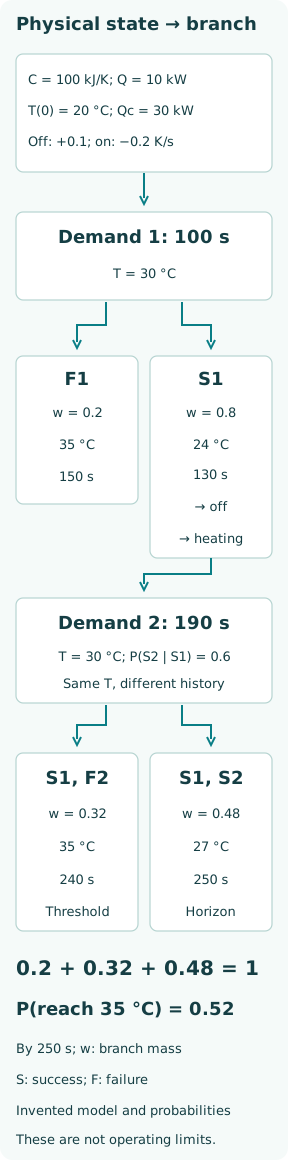
Use a hypothetical well-mixed inventory with heat capacity C = 100 kJ/K and constant heat input Q = 10 kW. Initially T = 20 °C and the cooler is off. A successful cooling start removes Qc = 30 kW; an unsuccessful start removes nothing. There is no inflow, outflow, phase change, ambient loss or delay. These simplifications make the trajectories exactly reproducible rather than suitable for an actual vessel.

The first upward crossing of 30 °C requests cooling. Successful cooling remains on until a downward crossing of 24 °C; then it switches off and a subsequent upward crossing can request it again. Failed starting leaves cooling unavailable for the remainder of the trial. Stop at first arrival at the invented 35 °C classification boundary, or at the 250 s horizon. Reaching the horizon below the boundary says nothing about unlimited future operation.

Derive the motion between switching events

MIT’s heated-tank lesson illustrates how a stated lumped energy balance becomes a temperature model. For the different closed-inventory model constructed here, C dT/dt = Q − uQc, where u is zero when cooling is off and one when it is on. Since 1 kW = 1 kJ/s, the slopes are +0.1 K/s and −0.2 K/s respectively.

Between events the temperature is linear: T(t + Δt) = T(t) + slope × Δt. Thus the first demand occurs after (30 − 20)/0.1 = 100 s. On a successful start, cooling reaches the reset temperature after (30 − 24)/0.2 = 30 s, at t = 130 s. This physical calculation determines the event times; a probability assigned to the start does not determine its thermal effect.

Use directional guards and retain the mode

An event condition needs more than the statement “temperature equals 30 °C.” Apply the start guard only while cooling is off, still available, and the temperature is moving upward. Apply the reset guard only while cooling is on and temperature is moving downward. A failed-start branch is a separate unavailable mode and must not request another independent start at every integration step.

The 30 °C start and 24 °C reset form hysteresis in this teaching logic. This avoids immediate start–stop switching at one boundary. The saved state contains time, temperature, cooler mode and demand history. If actuator delays, stored heat, maintenance or a continuously aging component are later added, their state variables must also be saved; otherwise two apparently identical restarts can have different legitimate futures.

Follow the repeated temperature rather than merging it

After the first reset at 130 s, warming from 24 °C to 30 °C takes 60 s. The second demand therefore occurs at 190 s. It has the same temperature as the first demand but a different time and history. If the second start succeeds, cooling resets at 220 s and the inventory warms to 27 °C at the 250 s horizon. A third demand would occur at 280 s, outside this calculation.

If the first start fails, the unchanged heating slope takes the inventory to 35 °C at 150 s. If the first succeeds and the second fails, arrival at 35 °C occurs at 240 s. Merging the two 30 °C nodes solely because their temperatures match would erase the demand count and alter the available continuation. Repeated physical values are not automatically equivalent probabilistic states.

Original thermal event sequence. From 20 degrees Celsius, heating at 0.1 kelvin per second reaches the first 30 degree demand at 100 seconds. Failure mass 0.2 reaches 35 degrees at 150 seconds. Success mass 0.8 cools to 24 degrees at 130 seconds and returns to 30 degrees at 190 seconds. Second failure mass 0.32 reaches 35 degrees at 240 seconds; double success mass 0.48 reaches the 250 second horizon at 27 degrees. Terminal masses sum to one and threshold mass is 0.52. — Original finite-horizon dynamic tree. Arrows follow the energy balance and switching law; displayed masses use stipulated conditional start probabilities. The repeated 30 °C state retains its time and demand history. Temperatures and probabilities are teaching inputs, not equipment operating limits.

Attach conditional probability only where uncertainty branches

Stipulate first-start success probability 0.8. Conditional on first-start success and reaching the second request in the stated history, stipulate second-start success probability 0.6. The lower second value is simply part of the original trial definition; no wear mechanism or measured dependence is inferred. A real model would need evidence for its own history-dependent outcome law.

The first-failure leaf has mass 0.2. The first-success/second-failure leaf has mass 0.8 × 0.4 = 0.32. Double success has mass 0.8 × 0.6 = 0.48. These disjoint leaves sum to 1. The probability of reaching 35 °C by 250 s is 0.2 + 0.32 = 0.52. Reset and reheating are deterministic here; multiplying by extra “probabilities of crossing” would count the same uncertainty twice.

Keep termination, truncation and unresolved mass distinct

A branch that reaches the threshold is a completed classified outcome. A branch stopped at the horizon without reaching it is also classified, but only for that finite question. A branch discarded because it is computationally inconvenient is neither. Maintain separate totals for threshold, horizon, intentionally truncated and failed-to-solve paths, with parent-to-child mass conservation at every split.

Sandia’s dynamic-tree publication notes that finer uncertainty treatment increases the state space and can prompt probability-based truncation. For a bounded indicator such as threshold reached, discarded mass can bound the uncomputed contribution: retain it as unresolved rather than silently renormalizing the surviving leaves. A simulation crash is not evidence that its path is safe or has zero probability.

Check event localization as well as integration accuracy

The exact piecewise-linear solution gives independent test targets: demands at 100 and 190 s, successful resets at 130 and 220 s, and threshold arrivals at 150 or 240 s. Integrate each segment and locate a crossing inside the numerical step. Carry the continuous temperature into the next mode at the event time; snapping only the displayed temperature while losing elapsed energy can conceal an implementation error.

Repeat with successively smaller maximum steps and tighter event tolerances. Compare event order, event times, final temperature, leaf classes and conserved mass, not merely a smooth-looking curve. A coarse step can jump over both a guard and a consequence boundary; the earliest valid crossing must be resolved first. This simple model permits exact localization, so a residual time-step effect identifies a numerical or guard-handling problem rather than physical uncertainty.

Separate model resolution from uncertainty in the inputs

Changing solver tolerance tests the numerical representation. Changing heat capacity, heat input, cooling capability, switching delay or conditional start probabilities tests the physical or probabilistic assumptions. Report them separately. A perfectly converged solution can still be wrong for equipment with stratification, temperature-dependent heat removal or a sensor that does not measure the modeled bulk temperature.

Also inspect simultaneous-event rules. If a shutdown, a reset and a terminal condition coincide, define which physical actions actually occur and how classification is evaluated. Do not let internal ordering of a software event list decide that question accidentally. For this example, first arrival at 35 °C terminates the path; neither post-threshold recovery nor its consequences are modeled.

Preserve an auditable chain from state to outcome

For each node, retain the parent identifier, incoming mass, complete restart state, active event guards, branch outcomes and their conditional probabilities. For each terminal path, retain its stopping reason and the trajectory sufficient to reproduce the classification. A path summary without temperatures and times cannot show whether a cooling demand truly occurred before the consequence.

Accept this example only when the energy balance, the exact event schedule, the three-leaf partition and the finite-horizon wording agree. For an engineering application, replace the teaching inputs and switching law with validated plant behavior, evidence-based uncertainty and justified consequences. The distinctive benefit is a traceable explanation of how feedback creates the next demand, including when the process revisits a familiar temperature in a materially different state.