Knowledge / Risk analysis methods
Coupled deviations in HAZOP: a multivariable safe operating envelope
Derive a two-variable thermal region, expose an unsafe corner hidden by separate limits, and distinguish steady feasibility, transient response and uncertainty margins.
On this page
A list of acceptable temperatures and acceptable flows can be misleading when each limit was checked while the other variable remained at its nominal value. The combined operating point may violate the physical condition those limits were meant to protect. A useful HAZOP review therefore asks which combinations are admissible, how the process moves between them, and which measurement uncertainties could move the true condition outside the assessed region.
Begin with the physical constraint behind the limits
An operating envelope is a set of permitted combinations for a defined duty, mode and consequence. Its boundary should come from equipment capability, process behavior and justified acceptance criteria. It is not necessarily a rectangle, and its meaning can change during startup, shutdown or equipment unavailability. A displayed variable being “within range” is meaningful only with the conditions used to establish that range.
This article uses a hypothetical nonreactive liquid heater to illustrate the geometry. The chosen outlet-temperature bound is an analytical constraint, not an instruction for a real vessel. Actual safety assessment would need material properties, local temperatures, pressure behavior and failure consequences beyond the lumped model. Keeping that distinction visible prevents a neat plot from acquiring more authority than its underlying evidence.
Build a balance with two independently described inputs
Let mass flow m enter a perfectly mixed heater at Tin and leave at bulk temperature T. Inlet and outlet flows are equal, so inventory remains constant. Take specific heat cp = 4 kJ/(kg K), external heat input Q = 40 kW and thermal capacity C = 200 kJ/K. Neglect reaction, phase change, ambient loss, wall storage and transport delay. Heat input remains fixed when flow changes.
MIT’s heated-tank lesson derives temperature dynamics from accumulation, stream enthalpy and heat transfer. For the original simplified heater here, C dT/dt = m cp(Tin − T) + Q. With m positive, the steady outlet is Tss = Tin + Q/(m cp). Flow and inlet temperature appear in the same expression, so separate checks cannot in general establish every combined condition.
Derive the admissible region rather than guessing a rectangle
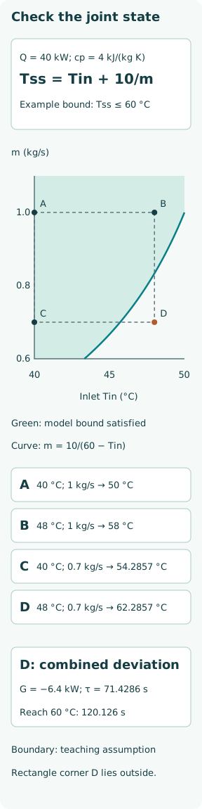
Choose the illustrative constraint Tss ≤ 60 °C. Since Q is positive, the steady admissible region requires Tin < 60 °C and m ≥ 40/[4(60 − Tin)] = 10/(60 − Tin) kg/s. Warmer inlet fluid leaves less temperature rise available for the same heat input and therefore requires greater flow in this model.
An equivalent heat-balance margin is G = m cp(60 − Tin) − Q, in kW. G ≥ 0 means that at the boundary temperature the flowing stream can remove at least the imposed heat input; G < 0 means temperature is still driven upward there. This sign test describes only the defined thermal condition. It does not establish mechanical integrity or cover an unmodeled fault.
Expose the corner that single-variable checks miss
The baseline Tin = 40 °C and m = 1 kg/s gives Tss = 50 °C. Raising only Tin to 48 °C gives 58 °C, below the chosen bound. Reducing only m to 0.7 kg/s while retaining the baseline inlet gives 54.2857 °C, also below it. It would be tempting to record separate limits Tin ≤ 48 °C and m ≥ 0.7 kg/s from those two tests.
At their combined corner, however, Tss = 48 + 40/(0.7 × 4) = 62.2857 °C. The heat-balance margin is −6.4 kW, whereas the baseline, warm-inlet-only and low-flow-only margins are +40, +8 and +16 kW. Both displayed inputs can satisfy the independently chosen rectangle while the combination violates the thermal constraint. At Tin = 48 °C the actual model boundary requires m = 0.833333 kg/s.
Turn the combination into a traceable HAZOP scenario
IEC 61882’s official description identifies guide-word examination as the basis of the HAZOP study process. In this original case, examine “more inlet temperature” while explicitly stating the low-flow operating condition, then link the “less flow” row back to that same combined scenario. This preserves the cause–condition–consequence chain rather than creating two disconnected recommendations.
Ask whether one cause can produce both changes, whether one variable is an intended operating choice, and how long they can overlap. For example, a specified reduced-throughput mode can coexist with warmer incoming liquid without requiring two simultaneous component failures. Conversely, merely multiplying two guessed occurrence probabilities would not establish independence. The combination needs a credible route into the state, not an assumption that every possible pair is equally likely.
Distinguish an eventual excursion from its timing
Assume the heater starts at the baseline steady 50 °C and both inputs step to Tin = 48 °C and m = 0.7 kg/s at t = 0. The new time constant is τ = C/(m cp) = 71.4286 s. Temperature follows T(t) = 62.2857 + (50 − 62.2857) exp(−t/71.4286), using the unrounded values in the calculation.
Solving T(t) = 60 °C gives t = 120.126 s. Thus the steady operating point is outside the region immediately after the input change, while the inventory takes time to reach the output constraint. This distinction matters for detection and response. It does not make a planned period outside the assessed region acceptable: delays, initial temperature and the actual consequence criterion must be justified separately.
Check a conservative rectangle against bounded errors
A rectangular rule can be conservative if its entire intended domain is inside the physical region. For example, with Tin ≤ 48 °C and m ≥ 0.85 kg/s, the worst nominal corner has G = +0.8 kW. This is a geometric observation under the stated model, not a proposed plant alarm or operating setting. For warmer inlet or greater heat input it would need reassessment.
Now suppose the indicated inlet can understate true temperature by 1 K, indicated flow can overstate true flow by 0.03 kg/s, and actual heat input can exceed nominal by 2 kW. At the same indicated corner, the bounded worst case gives G = (0.85 − 0.03) × 4 × (60 − 49) − 42 = −5.92 kW. With these simultaneous bounds and exact cp, the indicated-flow boundary at indicated Tin = 48 °C becomes 42/(4 × 11) + 0.03 = 0.984545 kg/s.
Keep uncertainty margins and protective timing separate
The bounded calculation is a worst-case construction, not a confidence interval or a probability of failure. It requires credible error bounds and a model valid across their range. Calibration error, changing fluid properties, heat-load uncertainty and unmeasured stratification need different evidence; one arbitrary blanket percentage does not explain them. If the variables are physically constrained together, use the justified joint domain rather than inventing impossible corner combinations.
HSE’s control-system guidance identifies response speed and margins between operating limits and system settings as protective-performance considerations. For this example, a protective action would have to change the energy balance soon enough to prevent the defined excursion. Detecting an input pair, issuing a command, achieving actual heat reduction and removing residual stored heat are separate parts of that response.
Verify the region, the path and the implementation
Check selected boundary points by substitution into the balance and test points on both sides. Verify that increasing inlet temperature or decreasing flow changes G in the expected direction. For the ideal model, a state starting at or below 60 °C cannot cross upward while G remains nonnegative continuously, because its temperature derivative at that boundary is nonpositive. That statement relies on the complete differential model and continuous input condition.
For an implemented envelope monitor, test units, signal age, bad-quality inputs, interpolation between tabulated points and the sign of the final comparison. A map of steady operating points cannot by itself validate a sensor location, an actuator or safe behavior during a mode transition. Use a protected test environment and retain the observed physical response, not only a screen image showing that an alarm appeared.
Close the finding with the assumptions attached
The HAZOP record should identify the combined inputs, relevant operating mode, physical constraint, causal route, estimated timing and the action that keeps the state within a justified region or takes it to a justified safe condition. Record which evidence supports the boundary and which parts remain conservative assumptions. Any change in heating duty, inventory, flow measurement or fluid properties can change the shape and timing.
The useful outcome is a reviewable relationship among variables, not a universal two-dimensional safety chart. Separate-limit checks remain valuable, but their corners and transitions need validation against the coupled model. In this example the overlooked condition is a warmer inlet combined with reduced flow; its significance is demonstrated by energy conservation before any risk score or protective-layer credit is assigned.