Knowledge / Risk analysis methods
HAZOP of recycle loops: composition deviations, impurity buildup and purge
Derive steady and transient impurity buildup in an original recovery loop, then turn the balance into HAZOP rows with explicit sampling and purge assumptions.
On this page
A recycle loop may keep the same indicated level and an apparently healthy circulation rate while its composition drifts for days. Recycle returns material; only a genuine outlet removes an impurity from the overall boundary. HAZOP therefore needs the component balance as well as the flow diagram. The important deviation can be delayed accumulation after an ordinary purge restriction, rather than an immediately visible loss of bulk flow.
State which material the loop is intended to retain
The design intention in this example is to recover useful carrier while preventing a retained impurity from building up in a circulating liquid inventory. Define the impurity chemically in a real study: “total contamination” is not enough to establish volatility, corrosivity, catalyst effects or compatibility. A species harmless in one duty may invalidate a separation or a product specification in another.
The University of Michigan HAZOP tutorial organizes the review around a parameter and guide word, followed by causes, consequences, safeguards and recommendations. Here the chosen parameter is composition in the recovery loop. Bulk flow, purge flow, product purity and sample representativeness are linked causes or evidence; they are not interchangeable measurements of that composition.
Draw an overall boundary that contains the recycle
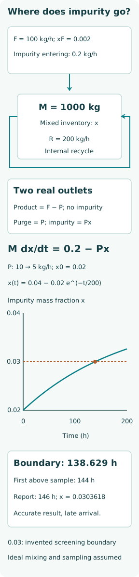
Consider a hypothetical 1000 kg well-mixed recovery-loop inventory. Fresh feed F = 100 kg/h contains impurity mass fraction xF = 0.002, so impurity enters at 0.2 kg/h. A selective separator withdraws an impurity-free carrier product. A nonselective purge P removes liquid at the inventory mass fraction x. The internal recycle R = 200 kg/h is entirely inside the balance boundary; line holdup and transport delay are neglected.
For this construction, product withdrawal is adjusted to F − P, holding the total inventory constant. At P = 10 kg/h the carrier product is 90 kg/h; at P = 5 kg/h it is 95 kg/h. This inventory-control assumption is essential. If product withdrawal stays fixed after a purge change, the inventory changes too, and the simple constant-M equation below is no longer sufficient.
Derive impurity removal without counting recycle twice
LearnChemE’s recycle-and-purge balances distinguish separation from a nonselective split, whose daughter streams retain the splitter-feed composition. For the different original lumped loop here, impurity accumulation is M dx/dt = F xF − P x. There is no reaction and the carrier product contains no impurity. Internal recycle appears once entering and once leaving a whole-loop balance, so its terms cancel.
A purge percentage needs a denominator. If purge and recycle are branches of the same splitter, the example’s baseline fraction is P/(P + R) = 10/210 = 0.047619; after restriction it is 5/205 = 0.024390. Neither number is P/F. Increasing R while holding actual P fixed does not change this ideal overall impurity-removal rate, although it can change real mixing, transport and separation performance.
Calculate the steady composition and the accumulation time
For constant positive P, the steady balance gives xss = F xF/P and the time constant is τ = M/P. At the original 10 kg/h purge, xss = 0.02 and τ = 100 h. These quantities answer different questions: the steady fraction describes the eventual composition, while the time constant describes how quickly the inventory approaches it after a disturbance.
Let purge fall to 5 kg/h at t = 0, starting from x0 = 0.02. The new steady fraction is 0.04 and the new time constant is 200 h. Solving the balance gives x(t) = 0.04 − 0.02 exp(−t/200), with time in hours. At 100 h, x = 0.0278694. An unchanged level and continuing 200 kg/h circulation do not contradict this rise: the reduced purge removes less impurity while extra pure-carrier withdrawal balances the total mass.
Put a delayed consequence on the HAZOP timeline
Choose x = 0.03 solely as an invented composition-screening boundary. Setting 0.03 = 0.04 − 0.02 exp(−t/200) gives t = 200 ln(2) = 138.629 h. The consequence is delayed by several operating shifts. A short observation after maintenance might therefore show normal composition even though the new operating condition is moving toward an unacceptable screening result.
If purge is completely lost, the model instead gives x(t) = 0.02 + 0.0002 t and reaches 0.03 in 50 h. This linear law is only valid while the assumed pure-carrier withdrawal remains feasible. It must not be extrapolated to an impurity fraction above one, or treated as evidence that a real separator continues operating unchanged at high contamination. A physical hazard threshold would need separate chemical and equipment evidence.
Apply more, less and other-than to composition explicitly
“More impurity” has a concrete chain: restricted purge → lower impurity removal → increasing x → eventual screening exceedance. Candidate causes include an obstructed purge line, wrong routing, reduced downstream capacity or a mistaken purge-ratio calculation. In a real system, demonstrate the next physical consequence instead of appending “fire” or “explosion” to every elevated concentration.
“Less desired carrier” is the complementary composition change in this two-component model; it can affect product recovery without adding an independent failure. “Less impurity” alone has no adverse consequence established here and should be recorded as such, rather than forcing a hazard. “Other-than specified impurity” addresses wrong feed or cross-contamination: the same total mass fraction can represent a different substance, for which this scalar balance still conserves mass but cannot establish chemical acceptability.
Test whether sampling can reveal the deviation in time
Assume ideal instantaneous representative samples every 24 h from t = 0, with a fixed 2 h reporting delay. A sample at 120 h is still below the 0.03 boundary; the next sample at 144 h is above it and arrives at 146 h. By then the actual fraction is 0.0303618. An accurate laboratory result can therefore be too late for a decision that must precede the actual crossing.
For an illustrative earlier alert at 0.028, the model crosses at 102.165 h. The next sample is taken at 120 h and reported at 122 h; actual x then is 0.0291330. Only 16.629 h remains to the screening boundary under the continuing disturbance. That is a calculated interval, not proof of a workable response: confirmation, decision, valve movement, safe disposal and the subsequent composition trajectory still need to fit within it.
Challenge both the sample and the assumed outlet
The preceding timing calculation assumes no sampling bias, stale line volume, analyzer drift, detection limit or missed sample. A sample from a fresh-feed-rich pocket can understate the loop average; a different phase may hold most of the impurity. Identify the sampled phase, location, transport age and analytical species. A total-organics reading, for example, cannot automatically identify which compound is accumulating.
Likewise, a commanded-open purge valve does not establish mass removal. Verify actual flow, destination availability and the purge composition relevant to the balance. If the separator sends impurity into product, the term for impurity in product must be added; if deposition or reaction occurs, add those terms too. An apparent agreement obtained by adjusting P to absorb every unmeasured sink is not validation of the physical model.
Choose actions that address the accumulation mechanism
Possible actions to evaluate include a measured purge minimum tied to the impurity load, a representative composition trend, a response based on the remaining time, and a controlled reduction of impurity input. Each must be assessed for its own side effects. Raising purge can send more contaminated material to treatment, lose valuable carrier, disturb inventory control or exceed downstream capacity.
In the ideal model, returning purge to 10 kg/h makes the eventual fraction 0.02 again, but it does not instantly erase accumulated material. The recovery trajectory begins from the composition at restoration. A closure test should therefore verify actual removal and the decline in impurity, including how operation is constrained while the loop is still above its chosen criterion. A corrected valve position alone is incomplete evidence.
Document the species balance and revisit changes
IEC’s public description of IEC 61882 includes documentation and follow-up within the HAZOP procedure. For this case, attach the boundary drawing, species definition, balance, retained inventory, assumed outlets, sampling timeline and evidence behind the real consequence. Keep proposed actions distinct from installed and demonstrated safeguards; this calculation does not assign an independent protection-layer credit.
Revisit the review when feed composition, separator selectivity, recycle routing, purge destination, inventory size or sampling method changes. The durable finding is not a universal purge percentage. It is the traceable relationship between impurity entering, impurity actually leaving, the inventory that stores the difference, and the time available before a justified composition boundary is reached.