Knowledge / Risk analysis methods
Non-coherent fault trees: success conditions and complemented events
Test failure monotonicity with a complete Boolean example, distinguish prime implicants from a chosen cover, and calculate complemented-event probabilities without treating opposite states as independent events.
On this page
An ordinary failure-only AND/OR tree assumes that adding a component failure cannot remove the top event. Some hazard definitions do not obey that assumption: an available energy source may enable one hazard while its loss enables another. The Boolean logic can still be analysed, but complements, state definitions and the quantification method must remain explicit. A larger list of failed components is no longer automatically a worse state for the particular top event.
Coherence depends on the declared state meaning
Let a basic variable equal 1 when the specified component failure is present and 0 when it is absent. Failure monotonicity means that changing any variable from 0 to 1, while holding the others fixed, cannot change the top event from 1 to 0. Weber’s fault-tree treatment makes coherence an explicit structural condition. A tree of positive AND/OR failure terms has this monotonic property.
A NOT symbol in an unreduced drawing is a reason to check the logic, not a sufficient final diagnosis. Complements can cancel during simplification, leaving a coherent function. Conversely, renaming “component works” as a new basic event can hide the complement visually without removing the underlying relationship. Test the reduced function against the actual state definitions.
A complement is the opposite state of the same event
If B means the primary source has failed in the declared snapshot, ¬B means that this failure is absent in that same snapshot. It is not a second independent component. The identities B ∧ ¬B = 0 and B ∨ ¬B = 1 are logical constraints, and P(¬B) = 1 − P(B) follows on the same probability basis.
“No recorded failure” is not necessarily the same as “verified functioning”. If the analysis distinguishes unknown, degraded or disconnected states, a binary complement may be too coarse. Define the sample space, operating mode and time basis before assigning a success condition. NASA’s handbook explains complementation and De Morgan’s rules; those rules preserve the stated event meaning, rather than supplying missing physical evidence.
A fixed house event is a different modelling choice. For one specified operating-mode calculation, define H = 1 when a maintenance bypass is deliberately selected and H = 0 when it is not. Substituting that fixed value includes or removes the corresponding branch; H is not an additional independent random failure. By contrast, B and ¬B in the example below are complementary random states within the same specified mode, with probabilities qB and 1 − qB. Setting ¬B permanently to 1 would assume B never occurs in that calculation and change the model. If mode occupancy itself is uncertain, model and justify that uncertainty separately rather than disguising it as a fixed switch.
Original example: two explicitly different undesired conditions
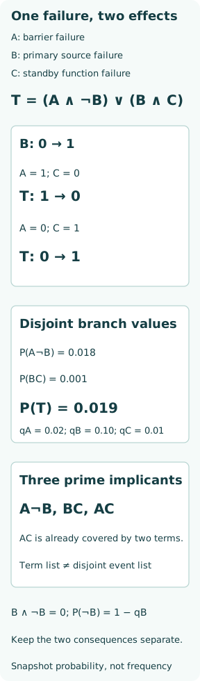
Consider a simplified snapshot model. A means an isolation barrier has failed; B means the primary energy source has failed; C means a required standby energy function has failed. Define an exposure condition E = A ∧ ¬B, where the barrier is failed while the primary source remains available. Define complete supply loss L = B ∧ C. The composite top event is T = E ∨ L = (A ∧ ¬B) ∨ (B ∧ C).
This deliberately combines two named undesired conditions to expose the logic. It is not a claim that exposure and supply loss have equal consequences, or a design recommendation for an actual energy system. Other barriers, sources, demands and dependencies are excluded. For decision-making, keep E and L visible separately even when their union is also reported.
The monotonicity test finds both directions of influence
With A = 1 and C = 0, changing B from 0 to 1 changes T from 1 to 0: losing the source removes the modelled energized exposure, while the standby function remains available. With A = 0 and C = 1, the same B change takes T from 0 to 1 because complete supply loss appears. Thus B is neither globally failure-increasing nor globally failure-decreasing in this function.
The complete eight-state truth table has T = 1 at (A,B,C) = (0,1,1), (1,0,0), (1,0,1) and (1,1,1). It is 0 in the other four states. This table also catches an important modelling error: adding a failure can remove this particular top event without making the whole machine safer. The conclusion depends on the chosen top-event boundary.
Prime implicants and a minimal cover are not identical lists
An implicant is a conjunction of state literals sufficient for T. It is prime when removing any literal would make it insufficient. For this example the prime implicants are A¬B, BC and AC. The first requires a failed barrier and a working primary source; a failure-only cut-set description would lose essential state information.
AC is also prime: with both A and C true, either value of B makes one branch true. Yet AC is redundant in the two-term cover A¬B ∨ BC, since AC = AC(B ∨ ¬B) is already covered. A complete list of prime implicants therefore differs from one irredundant expression. Neither list should be confused with mutually independent events when probabilities are calculated.
Worked probability: condition on B to obtain disjoint branches
Assume independent component states at one stated instant, with qA = 0.02, qB = 0.10 and qC = 0.01. Then P(E) = 0.02 × 0.90 = 0.018, and P(L) = 0.10 × 0.01 = 0.001. The branches are mutually exclusive because one requires ¬B and the other B. Therefore P(T) = 0.019, or 1.9%, and P(¬T) = 0.981.
Equivalently, condition on B: P(T) = P(T|¬B)P(¬B) + P(T|B)P(B). Independence makes the conditional probabilities qA and qC here. If component states are dependent, retain P(A|¬B) and P(C|B) rather than inserting the marginal values. None of these snapshot probabilities is a failure rate, annual event count or probability of ever entering T over a mission.
Two common shortcuts give two different wrong answers
Applying an independent-union formula to the two branches gives 1 − (1 − 0.018)(1 − 0.001) = 0.018982. That is too low: the formula invents an overlap of 0.000018 even though E ∧ L is impossible. Independent basic components do not make all derived branch events independent.
Summing all three prime-implicant probabilities gives 0.018 + 0.001 + 0.0002 = 0.0192, which is too high. AC overlaps A¬B by 0.00018 and BC by 0.00002; subtracting both restores 0.019. The INL technical reference cautions that complemented-event structures require an appropriate quantification method. Exact state enumeration, a correctly handled decision diagram or valid inclusion–exclusion preserves the logical exclusions.
Dropping a success condition changes the question
Replacing A¬B with A creates a different coherent model T* = A ∨ BC. With the same independent inputs, P(T*) = 0.02 + 0.001 − 0.00002 = 0.02098, about 10.421% above the actual example result. This may look conservative for the chosen number, but it erases the state mechanism and can distort importance and intervention decisions.
In the original model P(T) = qA(1 − qB) + qBqC, so ∂P(T)/∂qB = qC − qA = −0.01 for these values. Raising qB from 0.10 to 0.20 lowers the union to 0.018, but raises supply-loss probability from 0.001 to 0.002. That is not a reason to make the source less reliable. It shows why separate consequences and functions must accompany a composite probability.
Review the state logic before asking the software for a number
Document every literal’s meaning, the mode and time basis, dependencies, impossible combinations and all top-event branches. Check a truth table or equivalent state representation, including cases in which a failed component is restored. Confirm whether a reported term list is a complete prime-implicant set, a minimal cover or a solver approximation, and verify how complements and truncation are handled.
A static complemented-event tree represents conditions, not event order. If a hazard depends on which failure occurred first, repair timing, switching delays or memory, use a state-transition or other suitable dynamic model. The lesson of non-coherence is precise scope: Boolean algebra remains valid, but failure-only intuition and unexamined probability shortcuts do not.