Knowledge / Ship systems
Cooling-system heat balances: what can flow and temperature tell us?
A cooling-system heat balance compares the energy entering, leaving and accumulating inside a defined boundary. It can reveal whether measured or modeled flows and temperatures are mutually consistent. It does not identify the cause of a discrepancy without additional information. Energy balances and fluid properties are core topics in the DOE's public thermodynamics handbook. DOE thermodynamics handbook
On this page
Draw the boundary before doing arithmetic
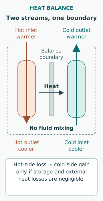
A typical marine central-cooling arrangement distinguishes seawater, low-temperature freshwater and high-temperature freshwater circuits. The fluids exchange heat through equipment such as coolers; they should not be treated as one mixed stream. The actual arrangement varies by installation. Wärtsilä central-cooling overview
For an initial calculation, choose one heat exchanger. Mark the hot-side inlet and outlet, the cold-side inlet and outlet, and any relevant heat loss to the surroundings. Record whether readings are simultaneous and whether operation is approximately steady. A temperature measured upstream of a mixing junction is not automatically the temperature at the exchanger inlet.
The useful simplified relationship
For a single-phase liquid with approximately constant specific heat, the heat carried by a flowing stream can be estimated as:
Heat-transfer rate = mass-flow rate × specific heat × temperature change.
If mass flow is in kg/s, specific heat in kJ/(kg·K), and temperature difference in K, the result is kJ/s, or kW. A temperature difference of 10°C is also 10 K. This equivalence is for temperature differences; equations requiring absolute temperature require an absolute scale, such as kelvin.
The relationship assumes the chosen heat-capacity approximation is suitable. Phase change, varying properties, additional energy terms and appreciable storage may require a fuller enthalpy balance. Heat-transfer behavior also depends on the exchanger and its temperature differences, not just on the energy carried by either stream. DOE heat-transfer handbook
A worked example with two water streams
Consider an invented teaching case with water on both sides. Use 4.18 kJ/(kg·K) as the stated approximate specific heat. These are not seawater design data or measurements from a vessel.
- Hot stream: 2 kg/s, cooling from 60°C to 50°C.
- Cold stream: 4 kg/s, warming from 20°C to 25°C.
The hot-side heat removal is 2 × 4.18 × 10 = 83.6 kW.
The cold-side heat gain is 4 × 4.18 × 5 = 83.6 kW.
With negligible heat loss and storage, the two sides agree. This is an energy-consistency check. It is not a demonstration that the exchanger has a particular surface area, fouling condition, pressure drop or capacity under every operating condition.
What if the readings do not agree?
Now change only the cold outlet reading to 24.5°C. Its apparent heat gain becomes 4 × 4.18 × 4.5 = 75.24 kW. The apparent difference is 8.36 kW.
That difference deserves investigation, but it does not uniquely diagnose a leak or a fouled exchanger. Check the time alignment, flow units, sensor locations, measurement uncertainty, property assumptions, heat lost elsewhere and whether temperatures are changing. A 0.5°C difference in this cold-side reading changes the calculation by 8.36 kW; the arithmetic itself shows why small measurement differences can matter.
Changing the outlet number simply to make the balance close would hide the question rather than resolve it. Keep the original readings and state any corrections and their basis separately.
Why transient operation looks different
After a load or flow change, fluid and metal can accumulate or release energy. In that interval, energy entering and energy leaving need not be equal at each instant. A stable final temperature also says little about how quickly the system reached it.
This is why a steady-state heat balance and a time-response model answer different questions. A time-response study additionally needs thermal inventories, initial conditions, suitable heat-transfer assumptions and a clear account of how inputs vary. Smooth animation or a plausible curve does not establish that these inputs are correct.
Convert the measured flow before using it
A volume-flow reading does not directly supply mass flow. The conversion is mass flow = density × volume flow, with compatible units and density appropriate to the actual fluid and conditions. A meter may also report a compensated reference volume rather than the physical volume at the measurement point. Record what the instrument reports before multiplying by a convenient water density. Additives and temperature can affect density and specific heat, so a freshwater teaching value is not automatically suitable for every coolant.
For an authored unit check, 36 m³/h equals 0.010 m³/s. With an explicitly assumed density of 1000 kg/m³, this becomes 10 kg/s. A 5 K temperature rise and assumed specific heat 4.18 kJ/(kg·K) then correspond to 209 kW. Using 36 as though it were kg/s would produce a different and unjustified result. The calculation demonstrates unit conversion, not the properties or approved performance of an installed circuit.
Energy consistency and heat-exchanger capacity are different
An energy balance can close even when a cooler has insufficient capacity for the required operating point. The balance states where energy goes; capacity also depends on the temperature driving force and thermal conductance. The archived DOE heat-transfer handbook develops the log-mean temperature-difference approach. It is educational thermodynamics, not a current marine design approval standard.
Using the earlier invented temperatures in an ideal counterflow arrangement, the two end temperature differences are 60 − 25 = 35 K and 50 − 20 = 30 K. Their logarithmic mean is (35 − 30)/ln(35/30) ≈ 32.44 K. If the same 83.6 kW duty were represented by Q = UAΔTlm, the implied UA would be approximately 2.58 kW/K. This result assumes the specified arrangement, steady conditions and an appropriate simple exchanger model. It does not separately identify area A and overall coefficient U, or prove a fouling diagnosis.
A small temperature difference amplifies uncertainty
The temperature difference is formed from two measurements. Their individual uncertainties, correlation and placement matter. For an invented uncertainty exercise, assume each temperature has standard uncertainty 0.20 K, the two errors are independent, and the measured difference is 5 K. The difference's standard uncertainty is √(0.20² + 0.20²) ≈ 0.283 K, or 5.66% of the difference. This is not the same as claiming an error of exactly 0.283 K.
If independent relative standard uncertainties for mass flow and specific heat are assumed to be 2% and 1%, a first-order combination gives approximately √(5.66² + 2² + 1²) = 6.08% for calculated duty. Shared calibration effects or correlated measurements would change that result. With a smaller temperature difference, the same absolute temperature uncertainty becomes a larger fraction. Consequently, an apparent imbalance should be compared with a justified uncertainty model before it is interpreted as physical missing heat. NIST’s propagation-of-error discussion explains the first-order method and the role of covariance.
Mixing and bypass flow can change what a sensor represents
Suppose, in a separate invented steady mixing example, 2 kg/s of water at 60 °C joins 1 kg/s at 30 °C. Assume equal constant specific heat, negligible heat loss and no phase change. The mixed temperature is (2 × 60 + 1 × 30)/3 = 50 °C. A sensor after the junction represents that mixture, not either incoming branch. Treating it as the hot branch's outlet would create an artificial heat-balance discrepancy.
This is why the fluid topology must accompany the readings. A bypass, recirculation path or mixing valve changes which flow and temperature belong together. Before diagnosing leakage or fouling, check sensor locations against the actual valve and connection state. A process diagram represents intended connectivity; field verification and controlled configuration records establish whether the operating system matches it. The arithmetic cannot repair a boundary drawn around the wrong streams.
Estimate thermal storage before assuming steady state
For a final authored example, assume a perfectly mixed inventory of 20,000 kg of water with constant specific heat 4.18 kJ/(kg·K). If heat input exceeds removal by a constant 1 MW, and metal storage and external losses are neglected, temperature rises at 1000/(20,000 × 4.18) ≈ 0.012 K/s, or 0.72 K/min. The model is only an initial-rate illustration; continuing that rate indefinitely would ignore changing heat transfer and operating limits.
A real circuit contains distributed fluid and metal inventories, transport delays and control responses. Measurements taken just after a load change may therefore disagree with a steady calculation even when energy is conserved. A practical investigation preserves time-stamped raw readings, identifies the boundary and operating state, checks units and properties, and separates measurement uncertainty from plausible storage or losses. Only after those checks should a specific fault hypothesis be compared against additional evidence.
Questions to ask of a result
- Which physical boundary does the balance cover?
- Are flow values mass flow or volume flow, and are units consistent?
- Are both streams and their properties identified correctly?
- Are readings synchronized and suitably located?
- Is energy storage negligible for the interval being interpreted?
- What measurement or model uncertainty could explain the residual?
A well-explained result retains these conditions beside the number. This guide is for understanding and checking a general calculation; changes to an operating vessel's cooling system require its approved technical procedures and qualified judgment.
Sources and related reading
Related library topics: pump curves and system resistance; measurement versus process state; steady-state and transient simulation.