Knowledge / Machinery and energy
Liquid-pipeline surge: wave speed and check-valve closure
Calculate elastic wave speed and a first Joukowsky surge, distinguish flow velocity from wave speed, and explain why reverse velocity at check-valve closure matters.
On this page
A liquid line can experience a large pressure excursion without any steam being present. If flow changes rapidly, the liquid compresses slightly and the pipe wall deforms. That disturbance travels as a pressure wave. The short event can load valves, supports and pump connections far above their steady-duty condition, or pull parts of the line toward vapour pressure.
Flow velocity and wave speed describe different motions
Liquid particles may move at a few metres per second while a pressure disturbance travels hundreds or more than a thousand metres per second. Wave speed a describes transmission of the disturbance, not the velocity of a parcel of water from the pump to the valve. Treating water as perfectly incompressible in a rigid pipe would eliminate the finite propagation time needed to describe this event.
KSB describes the pressure wave generated by rapid acceleration or deceleration. This article considers initially single-phase liquid. Condensation-induced hammer, gas-pocket compression and cavity collapse require additional physics; a single-phase result should not silently be extended into those regimes.
Both liquid stiffness and wall flexibility set wave speed
For a simplified thin-wall elastic model, use a = √[(K/ρ)/(1 + C KD/(Ee))]. K is liquid bulk modulus in Pa, ρ density in kg/m³, E pipe Young’s modulus in Pa, D internal diameter and e wall thickness in metres. C is a dimensionless restraint/Poisson-effect coefficient. It must match the actual structural assumptions rather than being treated as a universal constant.
DHI’s water-hammer theory includes the effect of fluid and conduit elasticity. For the illustrative calculation below, C is deliberately set to 1. The model excludes viscoelastic walls, entrained gas, flexible joints with unmodelled compliance and strong fluid–structure coupling. A selected software model should document how supports and axial restraint are represented.
Worked example: a 200 m liquid-filled line
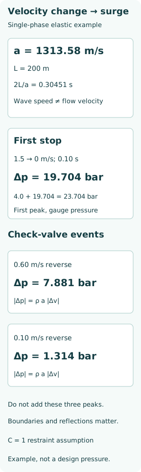
Assume ρ = 1000 kg/m³, K = 2.2 GPa, E = 200 GPa, D = 0.150 m and e = 0.006 m. Then KD/(Ee) = 0.275. The predicted wave speed is √[2.2 × 10⁶/1.275] = 1313.58 m/s. With a perfectly rigid wall, the same liquid model would give √(K/ρ) = 1483.24 m/s. Wall flexibility reduces the speed in this comparison.
For L = 200 m, the round-trip communication time is Tr = 2L/a = 0.30451 s. Consider a simple reservoir–pipe–end-valve system, initially flowing at 1.5 m/s, with an effective flow-stopping interval of 0.10 s. It is shorter than Tr, so the rapid-stop approximation is appropriate for an initial estimate before the returning reflection modifies the local state. The relevant interval is the change of flow, not merely actuator travel time.
Calculate the first pressure rise and its load scale
The Joukowsky pressure-change magnitude is |Δp| = ρa|Δv|. Stopping 1.5 m/s gives 1000 × 1313.58 × 1.5 = 1.97037 MPa, or 19.704 bar. With an assumed initial local pressure of 4.0 bar gauge, the simple first-rise estimate is 23.704 bar gauge. The surge increment is not itself the final absolute pressure.
The bore area is πD²/4 = 0.017671 m². Multiplying that area by the pressure increment gives 34.82 kN as the incremental pressure-force scale on a closed end. This is not a complete support or valve-body load calculation: pressure on all surfaces, momentum change, restraint geometry and dynamic response must be considered. Nor is the first-rise estimate a certified maximum for a network with reflections and several interacting events.
A check valve must respond to the reversing flow
After a pump trip, forward flow decelerates. A check valve that has not seated when flow reverses may allow reverse velocity to build. Arresting that reverse stream suddenly then generates another pressure disturbance. Calling a valve “fast-closing” gives too little information: its travel, inertia, spring action and hydraulic forces interact with the system’s deceleration.
Val-Matic’s dynamic-characteristic method compares system deceleration with reverse velocity at closure. It describes both early closure before appreciable reversal and deliberately controlled slow closure, subject to suitable system conditions. Selecting the quickest valve indiscriminately is not the same as selecting the best dynamic match.
Compare two stipulated reverse velocities
Keep the same liquid and wave speed. Suppose one assumed closure event arrests reverse flow of 0.60 m/s and another arrests 0.10 m/s. These are example inputs, not measured performance of any valve. The corresponding local pressure-change magnitudes are 7.881 bar and 1.314 bar. The sixfold difference follows directly from the sixfold difference in arrested velocity.
The sign and location of the resulting pressure excursion depend on which side of the closing valve is considered and the wave direction. Do not add these example increments automatically to the previous 19.704 bar rapid-stop case: they describe alternative stipulated events, not a timed sequence. A real transient model must establish when each wave arrives and how it interacts with the existing pressure field.
Slow travel does not guarantee a gentle flow change
Valve position and flow are not generally proportional. Much of the effective flow reduction can occur near the end of travel, even when the complete stroke lasts several seconds. A nominal closure time longer than 2L/a therefore does not by itself prove that the important velocity change is slow. The valve’s hydraulic characteristic and its time-dependent movement both belong in the boundary condition.
Wave reflections also depend on the boundary: a reservoir, closed end, branch, pump or gas vessel responds differently. Friction damps motion, but cannot be assumed to remove the first peak. A transient pressure minimum approaching vapour pressure may cause liquid-column separation; subsequent cavity collapse can generate a different, potentially severe event outside the initial single-phase estimate.
Mitigation must address the relevant event
Possible engineering measures include a suitable valve motion law, compatible check-valve dynamics, controlled pump run-down or a correctly sized surge device. Each changes a particular boundary or time scale. An air valve or pressure-relief device is not automatically protective under every combination of filling, shutdown and restart; opening and closing behaviour also matters.
Assessment should include normal stops, loss of power, simultaneous pump trips, restart and credible failure states. Use manufacturer dynamic data and pressure ratings at the actual temperature and duty. The illustrative peaks are not settings for relief valves, acceptance criteria for pipework or instructions to modify springs and dashpots in service.
Measure fast enough to see the event
A slowly logged gauge can show a normal pressure while missing a short transient. A useful investigation records sensor position, absolute or gauge reference, bandwidth, sample rate, trigger timing and synchronized valve/pump events. Choosing instrumentation requires the relevant rise time and wave travel times, not simply the normal process-control update interval.
The calculation sequence is therefore: establish the liquid and structural model, estimate wave speed and travel time, describe the actual velocity-changing boundary, then solve the event sequence and compare the resulting pressure/load envelope with equipment limits. Joukowsky is a valuable first calculation, but a check valve’s dynamic match and the complete network determine the final answer.