Load-sensing hydraulics: pressure margin, pump regulation and consumer interaction

Follow the highest-load signal, calculate the losses hidden in a common supply pressure, and distinguish normal pressure compensation from proportional sharing under pump saturation.

On this page

A load-sensing pump does not simply hold one fixed high pressure. It adjusts its displacement so that supply pressure follows a load signal with a defined pressure margin. That margin allows a metering opening to control flow. When several consumers operate together, the highest load, individual compensators and pump limits determine whether each function receives its requested flow.

The pump regulates a pressure difference to meet flow demand

In a simplified variable-displacement load-sensing arrangement, the pump controller compares outlet pressure with the load-sense signal. If the margin becomes too small as a metering opening increases, the controller increases displacement; if the margin becomes excessive, it reduces displacement. The load and the circuit establish the required pressure, while the pump supplies the flow needed to restore the controlled difference.

Danfoss describes the pump operating pressure as load pressure plus the LS differential. This does not make pressure independent of the actuator load. Maximum pressure control, maximum displacement, available shaft power and inlet conditions can all prevent the pump from satisfying the nominal margin.

The highest load is a signal, not the pressure at every consumer

A conventional multi-section LS network selects the highest active load signal, often through shuttle elements, and communicates it to the pump. The common supply must be sufficient for that load plus the needed margin and relevant losses. A lower-load consumer therefore receives oil from a supply pressure higher than it alone would require.

Individual pressure compensators can keep an intended pressure difference across each metering opening despite unequal loads, within their control range. Without suitable compensation, opening a lower-load path can divert flow and alter the speed of another function. Different valve architectures implement priority and compensation differently; the phrase “load sensing” alone does not define their behaviour under all limits.

Metering area and pressure drop jointly set flow

For a simplified turbulent orifice, Q =Cd A√(2Δpm/ρ). A is metering area, Cd a discharge coefficient, Δpm the pressure drop across that metering edge and ρ density. Holding Δpm approximately constant makes flow mainly responsive to area. This is why pressure compensation can make lever position a more repeatable speed command despite changing load.

The pump margin measured between pump outlet and LS port is not automatically identical to every local metering-edge drop. Line losses, compensator pressure drops and the signal architecture lie between those points. Parker’s P2/P3 catalogue distinguishes LS controls, bleed arrangements and response characteristics. Measurement locations and component definitions must be retained when comparing a real circuit with the simplified equations.

Worked example: two loads on one supply

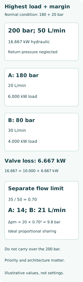
Assume consumer A requires 180 bar and 20 L/min, while B requires 80 bar and 30 L/min. Take tank pressure and line losses as negligible, and assume ideal compensation with a 20 bar nominal metering margin. The unsaturated common supply is then 180 +20 = 200 bar and total flow 50 L/min. These are illustrative values, not component settings.

Hydraulic power in kW is p[bar] ×Q[L/min]/600. Supply power is 200 ×50/600 = 16.667 kW. Useful hydraulic power delivered across A is 180 ×20/600 = 6.000 kW; across B it is 80 ×30/600 = 4.000 kW. Their sum is 10.000 kW. “Useful” here refers to actuator-port hydraulic power, before actuator friction or leakage.

The low-load branch still dissipates the pressure mismatch

For A, the ideal valve-path loss is(200 −180) ×20/600 = 0.667 kW. For B it is(200 −80) ×30/600 = 6.000 kW. Total valve dissipation is 6.667 kW, closing the balance 16.667 = 10.000 +6.667. LS operation reduces unnecessary supply relative to a higher fixed-pressure alternative, but does not eliminate the mismatch between simultaneous loads.

In the stipulated ideal compensation split, B’s 20 bar metering drop consumes 1.000 kW; its additional 100 bar compensation drop consumes 5.000 kW. With a separate assumed pump total efficiency 0.85, shaft input for this unsaturated state is 16.667/0.85 = 19.608 kW. Motor losses and return-line losses are excluded. These loss terms must not be counted a second time inside an efficiency already defined to include them.

Flow saturation changes what the margin controller can achieve

Now consider a separate case in which the same metering commands request 50 L/min but the pump can supply only 35 L/min. It cannot maintain every requested flow merely by receiving a higher LS signal. In an ideal proportional flow-sharing arrangement with no priority override, each branch receives the common scale factor 35/50 = 0.70: A gets 14 L/min and B 21 L/min.

Danfoss’s CLS100 operating principle describes a common reduction in metering margin when flow demand exceeds available pump flow. With unchanged area, coefficient and density, the orifice law gives the corresponding ideal metering drop 20 ×0.70² = 9.8 bar. This is a separate saturated condition: the earlier 200 bar supply and power balance must not be carried over unchanged without solving the actual circuit pressures.

Pressure compensation does not guarantee proportional sharing

Proportional sharing under saturation is an architectural feature, not a universal consequence of an LS pump. A circuit with independently pre-compensated sections, priorities or other special functions may allocate a shortage differently; a heavily loaded function can lose speed or stop while another continues. The exact valve version and schematic matter more than a broad family name.

Post-compensated flow-sharing designs commonly address this interaction, but even their ideal ratios are modified by spool characteristics, compensator limits, leakage, load checks and pressure limits. If one actuator reaches a pressure cutoff or an overrunning load requires a holding function, the simple two-positive-load example no longer describes the complete system. Safety-critical consumers may have an intentional priority that must be preserved.

Standby and transient response deserve separate attention

When no function demands work, a suitable LS arrangement can de-stroke and reduce supply pressure. That does not imply zero shaft power: control-oil flow, leakage and mechanical losses remain. A trapped or incorrectly vented LS signal can also prevent the expected low-pressure state. Signal-line volume, restriction and fluid compressibility affect how quickly the controller sees a changed demand.

Pump and valve response interact during sudden commands. Increasing margin can increase throttling loss and alter response; lowering it can reduce available flow through metering edges or make losses in the signal path more significant. The nominal 20 bar in this example is not an adjustment recommendation. Approved commissioning data, pressure limits and dynamic tests are required before changing any control setting.

Diagnose the pressure margin at the correct points

Record pump outlet, LS pressure, relevant work-port pressures, section flows, pump speed/displacement indication and oil temperature. Separate a flow shortage from pressure cutoff, leakage, a blocked LS path or an actuator load change. A single pump-pressure reading cannot reveal how flow is divided between consumers.

The central balance is common supply pressure set by the highest active requirement, local metering differences controlling flow, and finite pump capability limiting the result. Energy accounting then exposes the cost of pressure mismatch. A complete assessment must establish both normal regulation and the circuit’s intended behaviour when several functions compete for a limited flow supply.