Knowledge / Machinery and energy
Marine cable ampacity: grouping, ambient temperature and heat dissipation
Understand continuous cable current as a heat balance, trace grouping and ambient effects, and avoid applying rating-table factors outside their stated conditions.
On this page
The continuous current a cable can carry is not determined by conductor cross-section alone. Current produces heat; insulation, sheaths, supports and surrounding air must carry that heat away while the conductor remains within its applicable temperature limit. Closely packed circuits and a warm machinery space change the heat path. The same cable can therefore have different usable current ratings in different installations.
A current rating belongs to a defined installation
A complete rating statement identifies cable construction, number of loaded conductors, allowable conductor temperature, ambient conditions and installation arrangement. Free air, a covered tray, a conduit and a densely packed transit are not equivalent thermal environments. The hottest relevant part of the route can constrain the circuit even if most of its length has good cooling.
Prysmian’s North Europe marine catalogue states conductor temperature, ambient temperature and bunching assumptions alongside continuous ratings. Those footnotes are part of the rating, not optional background. A value copied without them can look precise while describing a different installation. The worked model below is deliberately synthetic and is not a replacement ampacity table.
From electrical loss to a conductor temperature
For a conductor segment, resistive heat is I²R. Per unit cable length, a simple three-loaded-core model gives q′ = 3I²R′, where q′ is W/m and R′ is the assumed effective resistance of each core in Ω/m. An effective thermal resistance Θ′ in K·m/W then gives θc − θa = Θ′q′. Here θc is the modelled hottest conductor temperature and θa the surrounding ambient.
Nexans’ general rating explanation links current capacity to electrical resistance, insulation thermal resistance and ambient conditions. A complete cable model separates the internal and external thermal paths, includes relevant sheath/armour and dielectric losses, and uses the applicable AC resistance. The single effective resistance used here compresses those details into a teaching model; it cannot determine the rating of a named cable.
Grouping changes the surroundings of each cable
Neighbouring loaded cables warm one another and reduce the exposed surface available for heat transfer. A cable in the middle of a bundle can see a different thermal environment from one at its edge. The relevant group includes circuits expected to carry current simultaneously, not merely a count of labels on the tray. Unloaded cables can still occupy space and alter airflow.
Grouping factors belong to a specified table and arrangement. If the base table already includes a permitted grouping condition, blindly applying another factor for that same condition can double-count it. Conversely, assuming that every bundle is covered by the base table can overstate capacity. Keep cable count, loaded-core count, spacing, tray arrangement and operating coincidence distinct.
Ambient temperature spends the available thermal margin
For a fixed conductor limit, warmer ambient leaves less temperature rise for the cable’s own losses. In the simple fixed-resistance model, current limit varies as the square root of the available temperature difference, not directly with that difference. External hot surfaces, steam lines or a poorly ventilated enclosure can create a local ambient unlike the compartment’s convenient thermometer reading.
The insulation’s maximum temperature and a published table’s calculation basis also need not be identical. A Prysmian marine catalogue explicitly uses an 85°C conductor basis in certain rating footnotes even though the cable supports 90°C. This is a specific catalogue example, not a universal marine limit. Read the construction-specific data and terminal limitations rather than selecting the highest temperature printed anywhere in the brochure.
Worked example: the same current in three heat paths
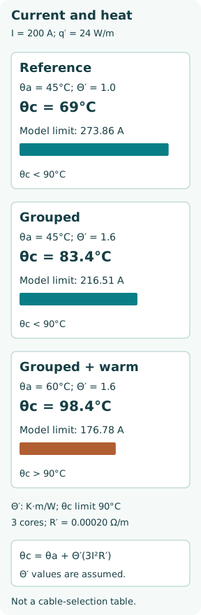
Assume three equally loaded cores, each with fixed effective resistance R′ = 0.00020 Ω/m. Use a teaching conductor limit of 90°C. In the reference installation let ambient be 45°C and effective thermal resistance Θ′ = 1.0 K·m/W. From 90 − 45 = Θ′ × 3I²R′, the model current limit is √[45/(1.0 × 3 × 0.00020)] = 273.86 A.
Represent a less favourable grouped arrangement by the assumed Θ′ = 1.6 K·m/W. With the same 45°C ambient, the model limit falls to √[45/(1.6 × 3 × 0.00020)] = 216.51 A. If that grouped route instead has 60°C ambient, it falls further to √[30/(1.6 × 3 × 0.00020)] = 176.78 A. The thermal resistances are invented; they do not correspond to a defined tray count, cable type or approved correction factor.
At a comparison current of 200 A, q′ = 3 × 200² × 0.00020 = 24 W/m. The three predicted conductor temperatures are 45 + 1.0 × 24 = 69°C; 45 + 1.6 × 24 = 83.4°C; and 60 + 1.6 × 24 = 98.4°C. Only the third exceeds the stipulated 90°C model limit. One unchanged current reading therefore does not demonstrate unchanged thermal margin.
Use correction factors consistently, not mechanically
In that same simplified model, the grouping factor is √(1/1.6) = 0.79057 and the ambient factor is √(30/45) = 0.81650. Their product applied to 273.86 A gives 176.78 A. The multiplication works because these particular factors were derived from the same separable model and reference condition. It is not proof that arbitrary factors from unrelated catalogues may be multiplied.
Actual rating methods may already incorporate conductor count, losses, grouping and installation assumptions. The product, governing rules and supplier instructions determine which corrections are independent. IEC’s current publication page identifies IEC 60092-352:2025 as the edition replacing 2005. An older catalogue can still explain its original calculation basis, but its tables alone do not establish compliance with a current project’s adopted edition and class requirements.
Loaded cores, harmonics and parallel paths need attention
A balanced three-phase cable may have three principal loaded conductors, but a neutral can carry substantial current under unbalance or certain harmonic conditions. Do not assume that a conductor is thermally irrelevant because its name is “neutral.” AC skin and proximity effects can make effective resistance differ from a simple cold DC value, and metallic coverings can add losses depending on construction and bonding.
Parallel cables also need more than an equal division of total current on paper. Impedance, length, connections, routing and mutual coupling influence sharing. One path can run hotter while a switchboard meter shows an acceptable total. The relevant evidence is the individual path loading and installation, assessed using the approved design method. The teaching example holds resistance fixed; a detailed solution couples resistance and temperature.
Continuous, cyclic and short-circuit ratings answer different questions
Continuous ampacity assumes the stated thermal condition can be sustained. A short duty may benefit from thermal capacity, but the starting temperature, pulse duration, repetition and cooling intervals must be known. A sequence of individually short events can accumulate heat. Short-circuit withstand is a separate high-current, short-duration assessment and does not define normal continuous capacity.
Ampacity is also separate from voltage drop, mechanical strength, fire performance, routing segregation and protective-device coordination. Passing one check does not waive the others. Protection must remain coordinated with the cable and application; a lower load forecast is not by itself a reason to change a protective setting. Actual selections and modifications require the vessel’s approved electrical design process.
Inspect the route as well as the current
A useful review records the exact cable specification, loaded cores, route segments, tray fill and spacing, transit/enclosure conditions, local heat sources, expected simultaneous loads and the rating method’s edition. Check terminations and connections separately: local connection heating is not fully described by a uniform cable-per-metre model.
Thermography or a surface temperature can help locate a problem, but surface temperature is not automatically conductor temperature. Interpret it with load, ambient, emissivity and the heat path. After adding circuits to a tray or enclosing a formerly open run, reassess the original assumptions. The durable lesson is that current capacity belongs to the cable and its surroundings together, and the limiting route section deserves explicit attention.