Knowledge / Machinery and energy
Marine ventilation fans: unstable flow, duct resistance and fan–system matching
Find the fan–duct operating point, interpret pressure and electrical power together, and distinguish stable curve movement from aerodynamic stall and system oscillation.
On this page
A ventilation fan does not deliver its nameplate airflow independently of the duct system. Its operating point is set by the pressure it can produce and the resistance of the complete flow path. On a ship, filters, louvers, dampers, bends and changing compartment conditions can move that point. Lower airflow can mean greater resistance, but unstable flow and increased electrical input require a more careful interpretation.
Use a consistent pressure and flow basis
A fan curve relates airflow to pressure at a stated rotational speed, density and configuration. A system curve expresses the pressure requirement of the connected path. Their intersection is a steady operating point when the stated assumptions apply. Aerovent’s fan-curve guide shows why flow, pressure, power and efficiency must be read together.
Keep total pressure and static pressure distinct. Total pressure includes the velocity-pressure contribution; a duct expansion can recover static pressure while losing total pressure. Fan total-pressure rise and a matching total-pressure efficiency form one consistent power basis. Combining a static-pressure reading with an unrelated total-efficiency value can produce a misleading power calculation. State where the pressure taps and flow measurement are located.
Resistance changes move the intersection
For a simple predominantly turbulent path with negligible fixed pressure offset, Δpsystem = kQ² is a useful approximation. Q is volumetric flow and k collects the effects of geometry and losses at the stated density. Closing a damper or loading a filter may increase the effective resistance, but the actual component characteristic should be used when the quadratic approximation is poor.
A shipboard system can also have imposed pressure differences from another fan, wind, stack effects or compartment-pressure control. Then a curve through the origin may be inappropriate. Branch flows must satisfy their own pressure balances; a correct total fan flow does not prove adequate ventilation at every required outlet.
Worked example: solve two assumed operating points
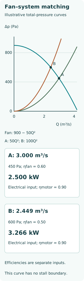
Use the invented fixed-speed fan total-pressure curve Δpfan = 900 −50Q², with pressure in Pa and Q in m³/s. It represents only a selected smooth branch, not a complete real fan or its stall boundary. For system A, let Δpsystem = 50Q². Equating curves gives 900 = 100Q², so Q = 3.000 m³/s and Δp = 450 Pa.
For system B, double the resistance coefficient to 100 Pa/(m³/s)². Now 900 = 150Q², giving Q =√6 = 2.449 m³/s and Δp = 600 Pa. Airflow falls 18.35% while pressure rise increases. The algebra predicts a different steady point; it does not claim that this particular change crosses an instability boundary. A measured manufacturer map is needed to locate that boundary.
Calculate air, shaft and electrical power separately
Air power on the chosen total-pressure basis is Pair =QΔp. For A, it is 3 ×450 = 1350 W. Assign total fan efficiency 0.60 and motor efficiency 0.90, with no separate transmission or drive loss: shaft power is 1350/0.60 = 2250 W and electrical input 2250/0.90 = 2500 W.
For B, air power is 2.44949 ×600 = 1469.69 W. Assign a lower fan efficiency of 0.50 at that point while keeping motor efficiency 0.90. Shaft power is 2939.39 W and electrical input 3265.99 W. Thus input rises 30.64% while airflow falls. The efficiency change is stipulated, not derived from resistance alone. A different fan’s power curve could show a different trend; motor current by itself is not a universal airflow meter.
Stall and surge are related but different behaviours
At unfavourable incidence, flow can separate from fan blades and reduce aerodynamic loading. Local or rotating stall concerns the blade/rotor flow field. A larger-scale oscillation involving fan pressure, duct flow and connected volume is a system instability commonly called surge. Stall can contribute to surge, but every noise fluctuation or local separation is not proof of whole-system flow reversal.
Greenheck’s vane-axial guide identifies a stall region and explains the risk of unstable operation as resistance increases. That evidence applies to the relevant fan configuration. It does not establish one universal minimum-flow percentage for all centrifugal, axial or mixed-flow fans. Operation should remain within the manufacturer’s stable envelope over the required range.
Curve intersection alone does not prove dynamic stability
A simple equilibrium sketch shows where pressures balance, but it does not contain blade separation, duct inertia, compressibility, control delays or multiple-fan interaction. Even the shape of a rising or flat segment must be interpreted with the system characteristic and dynamic model. The smooth decreasing curve used in the numerical example deliberately omits a stall region.
For a very limited one-state model, an increase in flow must create a restoring pressure imbalance to return to equilibrium: the local slope of fan pressure minus system pressure should be negative. That is a local quasi-steady criterion, not an aerodynamic stall test. A real fan can violate its allowable operating envelope even when this stripped-down slope test looks favourable.
Inlet distortion changes the fan, not just a distant duct loss
A close bend, obstructed inlet or swirling approach flow can make the rotor inlet nonuniform. Such installation conditions can reduce available performance relative to the laboratory curve. AMCA describes this as system effect at the inlet or outlet. Simply adding a generic length of straight-duct resistance may not represent the way the fan itself is being fed.
When investigating a shortfall, record the actual inlet/outlet arrangement, accessories, rotation, speed and density as well as filter and damper conditions. Raising speed to overcome a poor installation can increase power and stress without correcting the underlying flow quality. Changes near fire/smoke dampers or essential machinery-space ventilation also need the approved system constraints preserved.
Speed changes and parallel fans need their own checks
Under approximate similarity for the same fan, density and corresponding operating points, Q scales with speed n, pressure with n² and shaft power with n³. A separate 10% speed increase therefore gives nominal ratios 1.10, 1.21 and 1.331. These are similarity estimates with approximately unchanged efficiency, not a guarantee for a stalled fan or a system with a fixed pressure offset.
Parallel fans add flow at a common pressure only when their combined characteristics and branches support the assumed sharing. Unequal loading, reverse flow through an idle path and control interaction can alter the result. Check all intended combinations of operating fans and speed ranges, rather than approving only the all-fans-running design point. Motor, drive and mechanical speed limits remain independent constraints.
Diagnose with simultaneous flow, pressure and power evidence
Measure airflow at an appropriate traverse or calibrated station, identify static/total pressure correctly, and record speed, electrical input, density and oscillation timing. Inlet distortion can make a single-point velocity reading unrepresentative. A slowly averaged value can also conceal periodic instability; time histories may be necessary.
Then compare the actual condition with the relevant fan curve and system model. A stable shift caused by added resistance, a damaged or fouled rotor, installation system effect and a genuinely unstable operating point are different explanations. The useful conclusion comes from matching the fan to the complete installation and duty range, not from assuming that louder sound, higher current or a higher pressure reading means more useful ventilation.