Knowledge / Machinery and energy
Transformer thermal ageing: hot-spot temperature and variable loading
Distinguish winding hot spots from oil temperature, follow thermal lag, and integrate a changing ageing rate instead of using average load or average temperature.
On this page
A transformer can remain electrically functional while its solid insulation accumulates thermal damage. The relevant temperature is the hottest part of the insulation–winding system, which is not necessarily what a convenient surface or oil thermometer reads. Variable load adds a second difficulty: temperature has memory, and ageing is strongly nonlinear. This article explains the general thermal reasoning and uses a clearly identified mineral-oil/paper ageing model for its numerical example; the same numerical law must not be applied indiscriminately to dry-type marine transformers.
Define the insulation system before choosing an ageing law
Mineral-oil-immersed, ester-filled and dry-type transformers can use different insulation systems and temperature limits. Even paper insulation can be thermally upgraded or non-upgraded. A familiar reference temperature is not a universal maximum permitted winding temperature. The construction, declared insulation system, cooling mode and applicable loading guide must be identified first.
IEC’s public description of IEC 60076-7:2018 explicitly limits that loading guide to mineral-oil-immersed transformers. On a ship, a dry-type propulsion transformer may require a different basis. The following comparison therefore shows how to perform an ageing calculation once a suitable law is selected; it does not establish the permissible loading of an unspecified transformer.
Locate the hot spot within the heat path
Electrical losses generate heat in windings, core and other conducting parts. For an oil-cooled teaching model, a useful temperature decomposition is θH = θA + ΔθTO + ΔθH,TO: ambient temperature plus top-oil rise above ambient plus the winding hot-spot rise above top oil. All rises are temperature differences; degrees Celsius and kelvins have the same interval size. The final θH is a temperature value expressed in °C.
A top-oil sensor measures one part of that path. It does not directly establish the hottest conductor insulation temperature. A winding-temperature indicator may be a thermal model rather than a sensor physically installed at the hot spot. Direct fibre-optic sensing, where provided, also samples particular locations. Knowing what the measurement represents is as important as knowing its numerical value.
Variable loading produces losses and delayed temperature response
In a simple comparison with resistance held fixed, load-dependent copper loss varies as I²R. Raising current to 1.2 times its reference value raises that part of the loss to 1.44 times, not 1.2 times. Core loss, winding resistance change, eddy/stray losses and harmonic effects require additional treatment. A load percentage alone does not describe every heat source.
Heat capacity delays warming and cooling. Oil and winding hot spots do not necessarily share one time constant, and fans or pumps can change the eventual temperature and response. Consequently, identical current at two different times can coincide with different hot-spot temperatures. A recent overload followed by reduced load does not instantly restore the insulation to its earlier thermal state.
A simple lag calculation makes the memory visible
For an intentionally reduced first-order teaching model, let the hot spot start at 80°C and approach an assumed ultimate 140°C with time constant τ = 60 min after a fixed load/cooling change. Then θ(t) = 80 + (140 − 80)[1 − exp(−t/τ)]. The predicted temperature after 30 min is 103.61°C; after 60 min it is 117.93°C. At one time constant the model has completed about 63.2% of the temperature change.
The ultimate temperature and time constant are invented inputs. This is not the complete IEC or IEEE transformer thermal network, and 140°C is not presented as an acceptable operating value. Real analysis must use the installed transformer’s losses, temperature-rise test data, cooling arrangement and validated model. This small calculation simply shows why a new steady-state temperature cannot be assigned immediately after a load step.
Select a relative ageing rate, then integrate it
For the numerical comparison, adopt F(θH) = exp[15000/383 − 15000/(θH + 273)], with θH in °C. The constants use the conventional kelvin conversion and 110°C reference in this published relation. F is dimensionless and equals one at 110°C. ABB’s transformer-monitoring manual gives this form and distinguishes the treatment of insulation-paper types. Here it is used as an illustrative thermally upgraded-paper model, not a law for every insulation material.
Equivalent ageing time is the integral of F over elapsed time. For intervals with approximately constant temperature, use Leq = Σ Fi Δti. If Δti is in hours, Leq is equivalent hours at the model’s reference condition. Dividing by actual elapsed hours gives an equivalent average ageing factor. Neither quantity is automatically a remaining-life prediction: the initial insulation condition and other degradation mechanisms are still unknown.
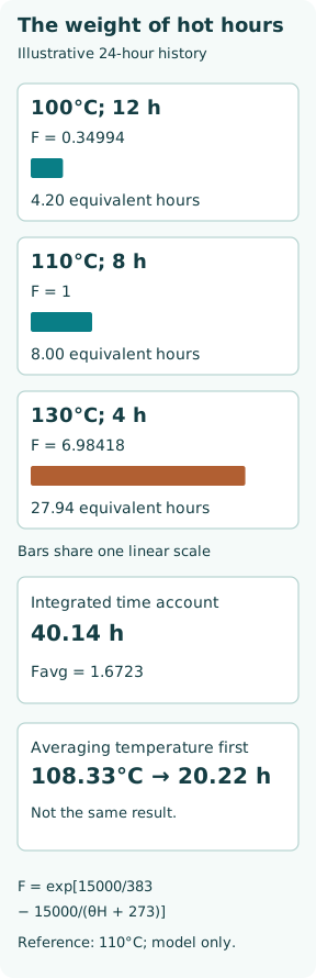
Worked example: four hot hours outweigh twelve cooler hours
Assume a measured-or-prescribed teaching history consisting of 12 h at 100°C, 8 h at 110°C and 4 h at 130°C. Treat each plateau as constant; transitions are deliberately omitted. The selected law gives F100 = 0.34994, F110 = 1 and F130 = 6.98418. The respective ageing contributions are 4.20, 8.00 and 27.94 equivalent hours.
Total equivalent ageing is 40.14 h over a 24 h period, giving an average factor of 1.6723. The hottest four hours contribute more than two-thirds of the calculated total, despite being only one-sixth of elapsed time. This result does not authorize that temperature history; it demonstrates the weighting produced by the chosen model.
The time-mean temperature is (12 × 100 + 8 × 110 + 4 × 130)/24 = 108.33°C. Applying the ageing law only to that mean gives F = 0.84268 and 20.22 equivalent hours. That shortcut would understate this example’s integrated ageing by almost half. Averaging temperature first and applying a nonlinear ageing law afterward are not interchangeable operations.
Cooling and moisture change what a thermal trend means
A blocked heat exchanger, fouled air path, failed fan or warmer cooling medium can raise temperature without an increased electrical load. Conversely, an effective cooling change may lower the hot spot at the same current. To compare days fairly, record the cooling mode and ambient or cooling-medium conditions as well as load. Rated kVA is tied to declared conditions, not an unconditional heat-removal capability.
Hitachi Energy identifies moisture in solid insulation as an important influence on paper degradation. Temperature-only ageing estimates therefore do not replace condition assessment. Moisture, oxygen exposure, contamination and prior deterioration can alter the relationship between a calculated thermal index and actual insulation strength. Cooling an aged transformer slows further thermal ageing; it does not reverse previously accumulated cellulose degradation.
Treat model uncertainty differently from temperature limits
Temperature measurement bias is magnified by the nonlinear ageing law. Missing a short hot period, using hourly averages during rapid transients or assuming that a failed cooling stage remains active can materially distort the accumulated result. The thermal model should retain its initial state across data intervals; resetting it to ambient repeatedly erases heat that is still present.
An acceptable cumulative ageing estimate also does not waive separate constraints on maximum temperature, oil/gas behaviour, accessories or mechanical condition. Thermal ageing and immediate equipment limits answer different questions. The approved operating envelope and protection functions remain controlling; a model should support engineering judgment rather than become an informal overload permission.
What belongs in a useful engineering record?
Retain the transformer construction and insulation basis, loading and ambient history, cooling state, sensor locations, thermal-model parameters, sampling interval and selected ageing equation. Report the hot-spot history separately from the accumulated equivalent hours. Show which intervals dominate the result and how missing data were handled.
The practical sequence is to identify the insulation system, calculate or measure its relevant temperature, preserve thermal memory and integrate the corresponding ageing rate. It is more informative than calling a transformer “lightly loaded on average.” Average demand can conceal a short, thermally expensive operating period, while a hot-spot estimate without a credible model can create false precision.