Knowledge / Machinery and energy
Variable-frequency drives: motor cooling, harmonics and low-speed limits
Relate motor speed, torque and heat to inverter waveform, supply harmonics and system efficiency without assuming that lower shaft power means lower thermal stress.
On this page
A variable-frequency drive changes how a motor receives electrical power and how it follows a process demand. That flexibility does not make every motor suitable for every speed or duty. Low-speed cooling, continuous torque, transient current, insulation stress and network interaction remain separate constraints. The useful unit of assessment is the supply–drive–cable–motor–load system, together with the supporting cooling and protection functions.
Separate electrical frequency from shaft speed
ABB’s drive-dimensioning guide describes induction-motor slip and distinguishes motor, converter and load requirements. For an induction motor with p poles, synchronous speed is ns = 120f/p in revolutions per minute when f is in hertz. A four-pole motor at 50 Hz therefore has synchronous speed 1,500 r/min. If its actual shaft speed is 1,470 r/min at a stated load, slip is (1,500 − 1,470)/1,500 = 2.00%.
At 10 Hz the corresponding synchronous speed is 300 r/min, but actual speed is not established by that number alone. Slip and the control method depend on load and motor characteristics. Nor is this relation a general speed law for every motor technology. Keep a displayed output frequency, an estimated speed and a measured shaft speed distinct when assessing performance.
Compare torque demand before comparing kilowatts
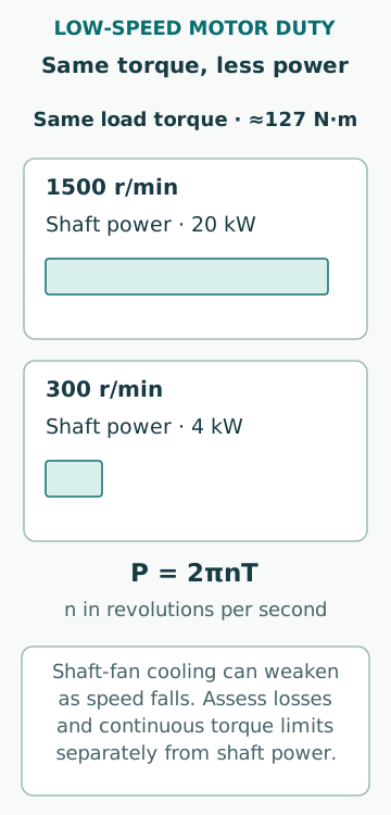
For an invented constant-torque duty, 20.0 kW at 1,500 r/min corresponds to T = P/ω = 20,000/[2π(1,500/60)], approximately 127 N·m. At 300 r/min, the same torque requires only 4.00 kW of mechanical output. The power falls to one fifth because speed falls, not because the required torque has fallen.
Motor heating therefore cannot be inferred from the shaft-power reduction alone. Torque-producing current, magnetizing current, electrical losses and cooling all matter. A constant-torque load is different from an ideal centrifugal load whose torque falls approximately with speed squared under suitable similarity conditions. Before expecting low-speed operation to be easy on a motor, identify which load relationship actually applies.
Check continuous low-speed cooling separately
ABB’s motor-loadability discussion explains that a shaft-fan-cooled induction motor can lose cooling capability as speed falls, limiting continuous low-speed torque. Separate cooling changes this boundary but has its own availability and duty. A short successful run does not prove that thermal equilibrium at a prolonged low-speed load will be acceptable.
The relevant evidence includes the motor’s permitted loadability curve, ambient conditions, enclosure, duty cycle and functioning cooling path. A drive’s electrical current capability may exceed the motor’s continuous thermal capability at the chosen speed. Conversely, a motor with adequate cooling does not make an undersized converter suitable. Check each constraint rather than using one nameplate kilowatt number as the answer for the complete operating range.
Use affinity savings only within their assumptions
The DOE part-load-efficiency tip sheet discusses drive efficiency together with speed-related load changes. For a separate ideal pump or fan example, assume geometric similarity, unchanged fluid properties, negligible static-head influence and a duty where shaft power scales with speed cubed. A 50.0 kW shaft demand at full speed becomes 50.0 × 0.80³ = 25.6 kW at 80% speed.
If the motor efficiency at that new point is assumed to be 92.0% and drive efficiency 97.0%, electrical input is 25.6/(0.920 × 0.970) = 28.7 kW, approximately. Those efficiencies are invented inputs, not universal values. Static head, changed operating point, minimum flow and auxiliary loads can alter system savings. The cube law is not a guarantee for every pump, constant-torque machine or complete ship service.
Distinguish fundamental frequency from switching pulses
The DOE motor–drive interaction note explains pulse-width-modulated output and the stress associated with rapid voltage changes and cable reflections. The low output fundamental frequency used to control speed is different from the much faster switching pattern. A motor can be turning slowly while its insulation is repeatedly exposed to steep voltage edges.
The relevant waveform at the motor terminals depends on the converter, cable and motor together. An ordinary meter reading of RMS voltage does not describe every peak or rise time. Compatibility assessment uses the actual motor insulation capability, drive output and installation evidence. Historical generic voltage or cable-length examples should not be adopted as universal limits for a modern marine installation.
Keep supply harmonics separate from motor-side stress
Eaton’s harmonics explanation relates harmonic voltage distortion to harmonic current and source impedance. Nonlinear input behaviour can therefore affect the shared electrical bus as well as the individual drive. The same current spectrum can produce different voltage distortion when the supply configuration changes. Generator operation and shore supply need their own verified network conditions.
Supply-side harmonic distortion is a different question from high-frequency motor-terminal pulses and common-mode current. A measure that addresses one may not address the others. Record where a waveform is measured, the operating load and source configuration, and whether the reported quantity concerns current or voltage. A drive described as low harmonic does not by that label alone establish motor insulation or bearing protection.
Read a harmonic-current example with the right denominator
Suppose a hypothetical periodic input current contains a 100 A RMS fundamental, 20 A RMS fifth harmonic and 10 A RMS seventh harmonic, with all other components and DC neglected. Current THD on a fundamental basis is √(20² + 10²)/100 = 0.2236, or 22.36%. Total RMS current is √(100² + 20² + 10²), about 102.47 A. Components at different frequencies combine through their squared RMS values under these assumptions.
This is neither a voltage-THD result nor a compliance assessment. In an ideal resistance that is equal at all three frequencies, the I²R loss would be 5.00% above the fundamental-only case because 10,500/10,000 = 1.05. Actual motors, cables and magnetic equipment have frequency-dependent losses, so that simple ratio cannot predict their full heating. The harmonic spectrum and equipment model remain necessary.
Assess bearing-current paths as a system
ABB Technical Guide No.5 treats high-frequency bearing currents through the complete common-mode path and describes distinct mitigation approaches. The appropriate choice depends on the actual current mechanism and installation. A vibration increase alone does not establish electrical erosion, and one insulated component does not automatically remove every possible path through the coupled machine.
Evidence may need to connect the observed damage pattern, operating history and suitable electrical measurements. Grounding, cable, filter and bearing arrangements must be coordinated with the equipment suppliers and applicable installation requirements. Improvised changes can relocate a current path or undermine another protective function. This discussion identifies the mechanisms to verify; it does not provide live electrical test instructions or authorize a grounding alteration.
Preserve the operating envelope through maintenance
A sound drive-system record names the motor and converter, load torque versus speed, continuous and transient duties, cooling dependencies, cable arrangement and relevant protection settings from approved documentation. It also identifies modes such as prolonged low speed, acceleration, braking and loss of a cooling service. A commissioning result at one steady speed cannot establish all those modes.
Common errors are equating low kilowatts with low motor heating, treating commanded frequency as measured shaft speed, applying pump cube-law savings to constant-torque loads, and assuming one harmonic or bearing solution is universal. The conclusion should identify which limits have supporting evidence and which still require assessment. Repairs or replacements must preserve the documented system compatibility rather than merely matching nominal motor power.
Sources
- Technical Guide No.7:Dimensioning of a drive system,RevC · ABB · Source check date: 2026-10-06
- Motor Systems Tip Sheet11:Adjustable Speed Drive Part-Load Efficiency · USDOE · Source check date: 2026-10-06
- Motor Systems Tip Sheet15:Minimize Adverse Motor and Adjustable Speed Drive Interactions,November2012 · USDOE · Source check date: 2026-10-06
- What is the Ohm’s-law explanation for harmonics? · Eaton · Source check date: 2026-10-06
- Technical Guide No.5:Bearing currents in modern AC drive systems,RevC · ABB · Source check date: 2026-10-06