Knowledge / Shipyards and ship structures
System cleanliness and flushing acceptance: sampling points, flow paths and residue evidence
Interpret flushing evidence through actual flow paths, sample identity and residual mass, with original velocity, mixed-volume and dead-leg examples.
On this page
A circuit can pass a pressure test and still carry debris into a sensitive component. Flushing asks where material can move and what evidence represents the wetted system. A clean sample becomes useful only after its location, operating state and relationship to unflushed branches are understood.
Define the cleanliness question before collecting a bottle
Pressure containment and internal cleanliness are different properties. A tight joint may enclose weld debris, fibres or preservation residues. Conversely, a low particle count says nothing by itself about pressure integrity. The acceptance question should identify the protected equipment, relevant contaminant and circuit boundary before a convenient sample point becomes the default definition of the system.
IACS introduces Recommendation 177 as machinery-piping quality guidance for construction and also repairs or modifications. That context helps place cleanliness within fabrication and commissioning. It does not establish one cleanliness number for every fluid service. A hydraulic servo, cooling passage and lubrication bearing can present different damage mechanisms and evidence needs.
Draw the temporary flow path as it actually exists
The flushing arrangement may bypass components, use temporary connections and divide the installed circuit into smaller paths. The relevant diagram is therefore a dated configuration, including open paths, isolated branches, temporary strainers and collection points. A line shown on the permanent drawing is not necessarily carrying flow during this particular operation.
Section 7.5 of the December 2023 recommendation addresses flushing preparation, vulnerable equipment and discharge evidence. Its scope and manufacturer precedence must be checked against the installation. Copying a generic fluid, speed or volume instruction without checking material compatibility and the real configuration would lose the connection between the procedure and its intended cleaning task.
Convert flow into local mean velocity
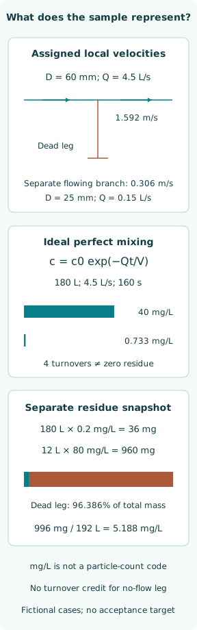
Assign a main line internal diameter of 0.060 m and volumetric flow Q = 0.0045 m³/s. The area is πD²/4 and mean velocity is v = 4Q/(πD²) = 1.592 m/s. These are fictional teaching values. The calculation says how an assigned flow relates to an assigned bore; it does not establish that every particle is mobilized or that the chosen velocity is suitable.
A separate branch with D = 0.025 m and Q = 0.00015 m³/s has v = 0.306 m/s. The main-line value cannot be assigned to this branch. Flow division, local geometry and the fluid condition matter. A total flowmeter reading can remain steady while a weakly supplied branch receives much less transport than its neighbours.
Use a mixed-volume model only where its assumptions belong
Consider an ideal, perfectly mixed volume V = 0.180 m³, initially containing a conserved contaminant at c0 = 40 mg/L. Clean fluid enters at 0.0045 m³/s and an equal outflow keeps volume constant. With no new source or deposition, V dc/dt = −Qc and c = c0 exp(−Qt/V). This is replacement flushing of a mixed volume, not a pipe plug-flow model.
After 160 s, 720 L have passed and Qt/V = 4 nominal turnovers. The predicted concentration is 0.733 mg/L. The initial 7200 mg becomes 131.873 mg, leaving 7068.127 mg removed in the model. Four turnovers do not mean zero residue; nor does this ideal curve describe deposits that detach late or a filter recirculation loop with a different mass balance.
Expose a dead leg with a separate residue snapshot
Now set aside that time history and assign a separate measured-looking snapshot: a 180 L main volume at 0.2 mg/L, plus a stagnant 12 L dead leg at 80 mg/L. The main contains 36 mg and the dead leg 960 mg. Total inventory is 996 mg, of which 96.386% is in the smaller branch. No claim is made that these concentrations arise from the preceding model.
If all 192 L were later mixed without loss or addition, concentration would be 5.188 mg/L. The clean main sample therefore cannot establish the dead leg's state. Repeating that same sample many times improves evidence about the sampled path, but does not create coverage of a hydraulically isolated region. The issue is representativeness before statistical precision.
Choose evidence that answers the relevant failure mechanism
A mass concentration in mg/L combines material without describing particle size, number or hardness. A particle-count cleanliness code carries different information and cannot be converted from these invented mass values without a particle population model. Dissolved chemicals, free water and solid fragments may each need different measurements. An apparently clear stream can still leave the wrong question unanswered.
The December 2023 Table 33 refers to ISO 4406 codes and gives manufacturer instructions precedence. This article does not reproduce those codes as universal targets. The project record should name the required property and accepted measurement method, together with the equipment specification that makes it relevant; an isolated laboratory number needs that interpretation chain.
Make sampling history part of the result
A sample belongs to a location, time and hydraulic condition. A bottle taken after settling can contain a different particle population from one obtained during active transport. A sampling tube can also retain material from an earlier state. Record enough configuration and collection information to distinguish a circuit result from a local pocket or sampling-device contribution.
A blank, duplicate or repeated sample can help investigate collection or analytical variability, but none automatically validates coverage of every branch. The main/dead-leg example makes that limit visible without assuming a particular laboratory procedure. If a result changes after a connection is disturbed, preserve both observations and their circumstances rather than averaging away a plausible release of stored residue.
Connect recovered residue to a bounded accounting argument
Debris caught on a temporary element is evidence that material reached that element. It does not directly quantify all material still upstream. Likewise, a declining collection rate can reflect depletion, reduced flow or a changed path. A useful comparison keeps inspected area, fluid throughput, collection interval and relevant equipment condition consistent or explicitly records the difference.
The mixed-volume example has a closed accounting balance because its assumptions include a conserved contaminant and measured-looking inputs with no uncertainty. Real residue accounting needs the same attention to sources and sinks: recontamination, inaccessible deposits, replacement fluid and sample removal. Missing terms should remain missing terms, rather than being silently interpreted as a successful removal balance.
Preserve cleanliness when restoring the operating circuit
A temporary bypass can protect a component during cleaning yet leave reinstatement as a new contamination opportunity. Opening flanges, replacing temporary elements and reconnecting instruments change the accepted boundary. The completion record should identify which portions were inspected or sampled before closure and what was subsequently disturbed, so the released configuration is the one the evidence actually describes.
This is configuration reasoning, not a valve-operating sequence. The approved work package must address isolation, compatible cleaning media, component protection and disposal for the actual vessel. A final photograph is useful for identity and arrangement, but cannot reveal a hidden branch concentration. Different evidence types should keep their own claims instead of being combined into an unexplained overall tick.
Close the acceptance argument without overstating the model
A coherent handover joins the circuit identity, dated temporary arrangement, branch coverage, measurement basis, results and reinstatement history. It states unresolved areas explicitly and connects any release decision to the applicable equipment and project requirements. Neither successful pressure retention nor a favourable main-line bottle alone establishes cleanliness throughout the installed system.
The original examples give three separate lessons: local velocity follows local flow and bore; perfect mixing predicts gradual concentration decay; and a small stagnant region can dominate residual inventory. None prescribes a production velocity, flushing time or acceptance concentration. Their value is to reveal what a measurement represents, what the mass balance assumes, and where additional evidence is still needed.
Sources
- IACS — New recommendation on shipbuilding quality of machinery piping systems. Official undated announcement; checked 8 October 2026 — Rec.177 scope: construction, modifications and machinery piping
- IACS Recommendation 177 — Shipbuilding and Remedial Quality Standard for Machinery Piping Systems. December 2023; official full 37-page text accessed 8 October 2026 — Scope §1; flushing §7.5 and Table 33, pp.36–37