Knowledge / Decision analysis
SAW / WSM: making a weighted total understandable
Author: Yönetici · Published:
Open the working calculator · Decision analysis
Imagine choosing between three suppliers. One is inexpensive, another offers better quality, and a third has stronger support. SAW, Simple Additive Weighting, also called the Weighted Sum Model, turns these competing considerations into an inspectable calculation. Comparable criterion values are multiplied by their weights and added. The largest total identifies the preferred alternative under the specified model.
This calculator uses one declared variant: benefit/cost min–max normalization followed by a weighted sum. SAW is not synonymous with a single normalization rule. Other transformations exist and can change the ranking. Vafaei, Ribeiro and Camarinha-Matos examine this issue; their study includes min–max normalization among the procedures assessed. Naming the chosen transformation is therefore necessary for reproducibility.
Prepare the decision before calculating
Put alternatives in rows and criteria in columns. A benefit criterion favors larger values; a cost criterion favors smaller values. Delivery time will normally be a cost, while durability will normally be a benefit. A criterion with a preferred target, such as temperature, needs an appropriate performance transformation before entering this simple increasing/decreasing framework.
Use nonnegative weights with a positive total. Normalize entered weights as w_j = a_j / Σa_j. A zero weight means that a criterion has no influence on the ranking. A weight is a modeling choice about trade-offs, not a discovered physical property. In this min–max variant, it governs the contribution of moving across the observed range of a criterion. Repeating nearly the same consideration in several columns can unintentionally count it several times.
Formula and worked example
Let x_ij describe alternative i on criterion j, with m alternatives and n criteria. Define L_j = min_i x_ij and U_j = max_i x_ij. For benefits, r_ij = (x_ij − L_j)/(U_j − L_j). For costs, r_ij = (U_j − x_ij)/(U_j − L_j). Calculate S_i = Σ_j w_j r_ij and rank in descending order.
Consider cost, quality and support with weights 0.40, 0.35 and 0.25. Alternative A has values (100, 80, 6), B has (120, 90, 8), and C has (90, 70, 5). Only the first criterion is a cost. The observed ranges are 90–120, 70–90 and 5–8. The normalized rows are A = (2/3, 1/2, 1/3), B = (0, 1, 1), and C = (1, 0, 0).
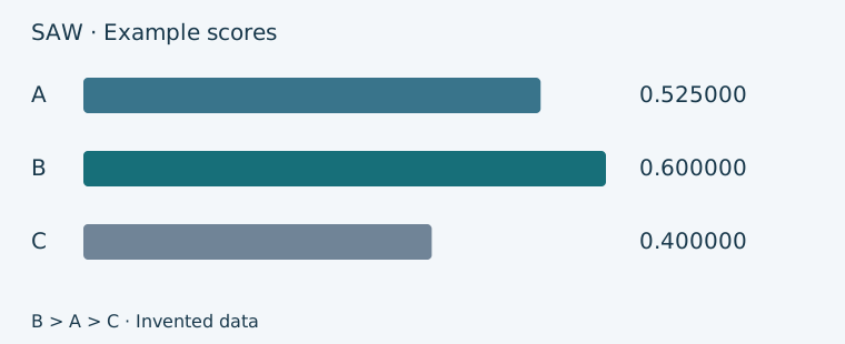
A's score is 0.40×2/3 + 0.35×1/2 + 0.25×1/3 = 0.525. B scores 0.600, and C scores 0.400. The resulting order is B > A > C. B is the most expensive option, but its quality and support compensate for that disadvantage. This illustrates a central assumption: a sufficiently good performance on one criterion can offset a poor performance on another. If a budget limit or minimum safety requirement is mandatory, screen alternatives against that requirement before applying this ranking.
What the result does and does not establish
Finite zero and negative values are mathematically usable in min–max normalization, provided they make sense for the criterion. A constant column produces a zero denominator. The proposed calculator convention assigns that column a zero contribution for everyone and reports the condition, without silently changing the remaining weights. If every positively weighted criterion is constant, all alternatives tie. A tie is a valid finding; forcing a unique winner would invent information.
The set of alternatives matters. Adding an extreme option can change a column's observed range and potentially reverse the relative order of existing options. Conversely, multiplying a whole column by a positive constant or adding the same constant to every value leaves its min–max values unchanged. These are algebraic properties of this variant, not permission to transform measurements without considering their meaning.
For a useful sensitivity check, increase the example's cost weight while preserving the quality-to-support weight ratio of 7:5. B and A tie when the cost weight reaches approximately 0.460674. Above that threshold, A can overtake B. This tells you more than merely reporting the original winner: the recommendation depends on how strongly cost is prioritized.
A score is not a probability, a success percentage, or a monetary benefit. Inspect weighted contributions, compare plausible weight scenarios, and test uncertain measurements. Rank using unrounded results and disclose any numerical tie tolerance. The linked calculator is most useful as a way to investigate these choices, rather than as an automatic substitute for judgment.
Source: Vafaei, N., Ribeiro, R. A., & Camarinha-Matos, L. M. (2022). Assessing Normalization Techniques for Simple Additive Weighting Method. Procedia Computer Science, 199, 1229–1236. https://doi.org/10.1016/j.procs.2022.01.156
Declared implementation rules
The calculator on this site accepts nonnegative data within a bounded teaching scope; nonzero values lie between 10⁻⁹ and 10⁹. Although the SAW formula supports a wider real-number domain, this interface does not accept negative observations. EDAS requires every value to be strictly positive. Weights must be zero or between 10⁻⁹ and 10⁶, with a positive total.
Test the example yourself
Recalculate with different matrix values and weights. Read the intermediate values alongside the sensitivity table.