The P–F interval: inspection spacing and time to act

Define the required function before drawing the curve

A seawater pump may continue rotating while its flow becomes insufficient for the heat load. In that case functional failure occurs before mechanical seizure. State the duty, operating envelope and performance criterion first: flow at a specified system condition, acceptable leakage, electrical insulation performance or another measurable requirement. A vague endpoint such as “broken” conceals the available warning time and changes the apparent success of the monitoring programme.

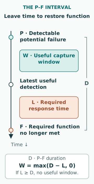
P is also a defined observation, not the first microscopic damage. A bearing defect may exist before a chosen sensor and processing method can distinguish it from background vibration. Changing the sensor location, threshold or technique can move P even when the physical damage history is unchanged. The NASA RCM guide, section 4.1, illustrates this connection between detectability and functional loss. Its facilities examples explain a concept; they do not set marine inspection intervals.

Separate warning time from usable intervention time

Let D denote the P–F duration and L the elapsed time needed after detection to confirm the finding, plan the work, obtain parts, arrange isolation, repair and verify restoration. The useful capture window is W = max(D − L, 0). Detection during the final L hours may be technically correct but too late to prevent the defined consequence. A remote laboratory result also has transport and reporting delays; the sample date is not the decision date.

The practical question is therefore whether the whole response fits inside the remaining interval. If a replacement is already on board, L may be short. If the same part requires an uncertain port delivery, L may dominate. Monitoring cannot compensate for a response that cannot be completed, although earlier information may still support an approved operating restriction or contingency. Those alternatives have their own evidence and authorization requirements.

Calculate an idealized capture probability

For an original teaching example, assume fixed D = 120 h, fixed L = 36 h, perfectly reliable inspections every T = 96 h, and potential-failure onset uniformly distributed relative to the inspection schedule. Then W = 84 h and the chance of an inspection within the useful window is min(1, W/T) = 84/96 = 87.5%. This is the probability of timely capture under the assumptions, not the probability of preventing every equipment failure.

If T is reduced to 48 h, the ideal timing calculation reaches 100% because every 84 h window includes an inspection. It does not establish a real guarantee: the inspector may miss the condition, the interval may shorten, or the response may be delayed. If L rises to 72 h while T remains 96 h, W falls to 48 h and capture falls to 50%. Better logistics can therefore improve the same monitoring programme without changing the sensor.

Add the chance of detecting what is present

A scheduled visit and a successful detection are different events. If exactly n independent opportunities exist and each has detection probability p, the chance of at least one detection is 1 − (1 − p)^n. Two opportunities at p = 0.80 give 96%. That independence is a strong condition: two readings at the same poor location, using the same unsuitable frequency band, may share the same blind spot.

Detection probability usually depends on defect size and operating state rather than remaining constant. A quiet unloaded machine may conceal a load-sensitive defect; access limitations may remove a measurement direction. Record whether the route was completed under a valid state. Do not count a postponed measurement, an invalid waveform or an inaccessible point as successful surveillance simply because a work order was closed.

Treat the P–F interval as a distribution

A fleet average of 200 h can hide a minority of failures progressing in 30 h. Choosing T from the average gives little protection against that fast subgroup. Organize evidence by failure mechanism, load, contamination, speed and repair condition. A single smooth curve is an explanatory sketch, not a record of all possible degradation paths.

When D and L vary, the ideal capture expression becomes an average of min(1, max(D − L, 0)/T) over credible cases. In a simple two-case illustration, let half the cases have W = 24 h and half W = 120 h with T = 72 h. Average capture is (24/72 + 1)/2 = 66.7%, although the average W is 72 h. Substituting the average window into the formula would incorrectly predict 100%.

Shorten intervals for a reason and retain escalation

Increasing the monitoring frequency after a credible change can reveal whether degradation is accelerating, but the additional reading must arrive soon enough to affect the decision. Compare changes against measurement scatter and matched operating conditions. A new slope after a load increase may be an operating effect; repeated growth at the same duty is different evidence.

An adaptive schedule needs a trigger, the next due time, an accountable reviewer and a latest decision point. “Watch closely” leaves all four unspecified. Escalation should also address missing data and unexpectedly fast change. Where the failure mechanism has no observable precursor, or develops faster than any feasible response, another maintenance or protective strategy is needed. More frequent measurements alone cannot create a useful P–F interval.

Include the laboratory and decision queue

A weekly oil sample does not create a seven-day detection system if the bottle spends four days in transit and the report waits another two days for review. For a condition becoming detectable just after a sample, the worst timing includes almost the entire sampling interval plus those delays. If the physical warning window is uncertain, quoting only the collection frequency can materially overstate protection.

Draw a simple time line with acquisition, dispatch, receipt, analysis, review, decision and completion. In a hypothetical case, the illustrative delays are 24 h from sampling to dispatch, 18 h in transit, 12 h for analysis, 6 h for review and decision together, and 30 h for work and restoration verification, totaling 90 h. A 72 h P–F interval would already be shorter than this response chain. Increasing collection frequency cannot by itself close the gap; identify which delays can actually be reduced.

Account for monitoring outages and competing failures

Continuous monitoring reduces the scheduled wait only while the entire measurement-to-response chain is available. A sensor with fresh power but a failed communication link may supply no usable warning. A dashboard displaying a last-known value can conceal the outage. Assess sensor health, timestamp age and alarm delivery separately from the machinery condition.

Finally, a route designed to detect progressive bearing damage does not cover every cause of pump loss. An electrical supply failure or sudden coupling damage can occur outside that mechanism’s P–F model. Keep a coverage statement listing the targeted mechanisms and the important uncovered ones. This makes the monitoring claim testable and prevents a successful bearing programme from being mistaken for complete system protection.

Learn from the full sequence

Retain the last valid normal observation, first abnormal indication, confirmation time, decision time, repair completion and demonstrated functional condition. These timestamps expose whether the limiting factor was detection, interpretation, logistics or work execution. They also distinguish a defect discovered during inspection from a failure whose onset was merely assumed to coincide with the inspection.

Review successful interventions as well as missed failures. Replacing every suspect item prevents observation of its eventual failure time, so the historical P–F sample becomes selectively incomplete. That does not justify running safety-critical equipment to failure to collect data. It means interval estimates need explicit uncertainty and supporting engineering evidence. The defensible result is a schedule linked to a particular mechanism and a feasible response, with clear conditions for revising it.

Sources

• Reliability-Centered Maintenance Guide for Facilities and Collateral Equipment · NASA · Source check date: 2026-10-06