Knowledge / Navigation and marine safety
Forecast uncertainty in weather routing: ensemble spread and decision windows
Preserve forecast-member identity along candidate routes, count the event that matters and determine whether the next update can arrive before a meaningful decision deadline.
On this page
A weather-routing decision depends on possible conditions along a moving vessel’s path, not just the forecast at one point or the smoothest-looking mean field. An original ten-member example separates ensemble spread, route-wide threshold screening and the time left to use another forecast. The calculations compare evidence; they do not select a real route.
Define the decision before reading the ensemble
State the candidate routes, expected passage times and ship-specific quantities relevant to the decision. Significant wave height, wave period, direction, wind and vessel response are different variables. ECMWF’s wavegram guide distinguishes significant wave height from maximum individual wave height. A threshold attached to one must not be silently transferred to the other.
Here the educational event is Hs > 4.0 m at either of two specified route gates. The threshold is invented for arithmetic and is not an operating limit. Gates are selected position–time samples on each route; they do not cover every point between them. Even a correct count therefore screens this defined event, not all weather exposure or vessel damage.
Understand what the spread represents
ECMWF describes ensembles as a way to represent uncertainty in possible forecast developments. Members reflect assumptions about uncertain initial conditions and modeling, rather than independently observed future worlds. Their spread is information about the model’s represented alternatives; it does not automatically cover every source of forecast error or local variability.
For the finite teaching set, mean μ = ΣHi/N and spread s = √[Σ(Hi − μ)²/N], with H in metres. The denominator is N, so this is the population spread of the listed members. A small spread means those members agree closely; it does not prove that they agree with reality. Verification is a separate evidential requirement.
Use a complete paired scenario set
The table supplies ten equally weighted fictional members. A1 and A2 are the two gates on route A; B1 and B2 are the corresponding two gates on route B’s own assumed schedule. Every row retains the same member identity across all four values. These are invented values for analysis, not downloaded weather or claims about an actual sea area.
This pairing allows the question “does this member exceed the threshold anywhere sampled on this route?” to be answered before averaging. Sorting each column independently or selecting a favorable member separately at each gate would create a synthetic journey that no member predicts. Both alternatives must also be evaluated at their own expected passage times, because different routes can encounter the same weather system at different stages.
| Member | A1 | A2 | B1 | B2 |
|---|---|---|---|---|
| 1 | 2.8 | 3.1 | 3.1 | 3.2 |
| 2 | 3.0 | 3.4 | 3.2 | 3.3 |
| 3 | 3.2 | 3.7 | 3.3 | 3.4 |
| 4 | 3.4 | 4.1 | 3.4 | 3.5 |
| 5 | 3.6 | 4.4 | 3.5 | 3.6 |
| 6 | 3.8 | 4.6 | 3.6 | 3.7 |
| 7 | 4.2 | 3.8 | 3.7 | 3.8 |
| 8 | 4.4 | 3.5 | 3.8 | 3.9 |
| 9 | 3.5 | 3.3 | 3.9 | 4.0 |
| 10 | 3.7 | 3.6 | 4.1 | 4.2 |
Compare equal means with different spread
At the first gate, both routes have mean 3.56 m. Route A’s spread is 0.473709 m and B’s is 0.303974 m, rounded to six decimals. Their first-gate exceedance fractions are 0.2 and 0.1. The same mean therefore hides a different distribution relative to the chosen threshold, even in this deliberately small scenario set.
At the second gate, means are 3.75 m for A and 3.66 m for B. All four gate means are below 4.0 m, yet individual members exceed it. Screening the mean alone would miss those members. A threshold applied after averaging is a different operation from averaging the member-level threshold outcomes, and the two operations do not generally commute.
Count the route event within each member
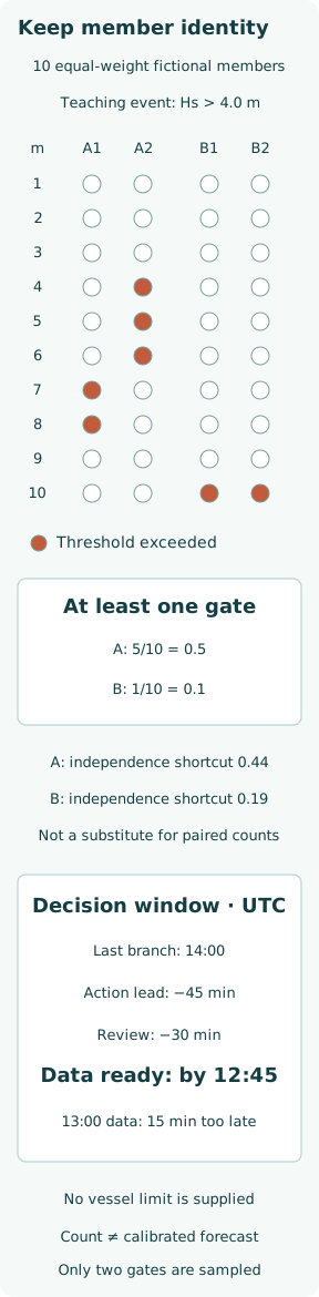
Define Im,r = 1 if max(Hm,r,1, Hm,r,2) > 4.0 m and zero otherwise. The route fraction is pr = ΣIm,r/10. For A, members 4, 5 and 6 exceed at the second gate, while 7 and 8 exceed at the first. Five distinct members therefore trigger the event, giving 0.5 for the sampled route.
For B, only member 10 exceeds, at both gates, giving 0.1 rather than counting the same member twice. The value 4.0 m in member 9 does not exceed a strict greater-than threshold. Defining the inequality is part of defining the event; changing to greater-than-or-equal would change the result. The native figure shows the member-level logic before the aggregate fractions.
Avoid an unsupported independence shortcut
ECMWF’s probability guidance explains why combined time or area events need member-level dependence. In A, gate fractions 0.2 and 0.3 would give 1 − (1 − 0.2)(1 − 0.3) = 0.44 under independence, while the actual paired count is 0.5. The exceedances occur in disjoint members, so the independence shortcut describes another joint model.
For B, both gate fractions are 0.1 and the shortcut yields 0.19, whereas their perfectly coincident member event gives 0.1. These opposite errors show that independence is not a generally conservative replacement. Correlation across time and space is part of the forecast trajectory; preserving it is essential when translating point forecasts into a route event.
Check calibration and finite-member limits
ECMWF’s reliability diagrams compare forecast probabilities with observed event frequencies over many cases. That comparison tests whether probabilities can be taken at face value in the relevant setting. A confident-looking narrow ensemble can still be systematically biased. Calibration also needs a representative variable, region, lead time and event definition rather than an unrelated aggregate score.
The ten-member exercise changes in increments of 0.1 when one member changes its event status. That coarseness is not an uncertainty interval, and zero exceedances would not prove zero real-world chance. The listed fractions are transparent scenario summaries, with no calibration data attached. Additional digits cannot turn them into validated probabilities of vessel damage or acceptable passage.
Keep the route comparison multi-dimensional
Under the chosen screen, B has fewer exceeding members. Assume separately that it adds 24 nautical miles at a constant 12 kn; its nominal extra duration is 2.0 h. This arithmetic does not include fuel consumption, currents, speed loss, arrival constraints or ship response. It exposes a comparison that would need those additional inputs rather than declaring B optimal.
An actual routing model may make speed and arrival time depend on the forecast member and chosen control policy. Then each trajectory must be sampled at its own resulting times. A fixed-time comparison can change when the vessel slows or a storm shifts phase. The educational table intentionally holds schedules fixed so that this additional feedback is not smuggled into the results.
Calculate the last useful update time
Suppose the last meaningful route branch is reached at 14:00 UTC on one fictional day. Allow 45 min for the action lead and 30 min for evaluating new data. The latest useful data-ready time is 14:00 − 45 min − 30 min = 12:45. This deadline is a decision assumption, not a meteorological forecast-valid time.
A new dataset that becomes usable at 13:00 misses that window by 15 min, even if its nominal model cycle began much earlier. Download, processing and review time matter as well as model initialization. Waiting for an update is useful only when the decision remains feasible after the update is interpreted; a later forecast cannot restore an already-lost alternative by itself.
Retain a conditional decision record
Record the forecast source and cycle, variable definitions, route timing assumptions, event threshold, member treatment and calibration limits. State what observation or new forecast would change the comparison and when that information could still be used. This creates a bounded reassessment process instead of treating each new weather map as an isolated reason to reverse the plan.
The original example yields route fractions 0.5 and 0.1 for its two-gate event, equal first-gate means with different spreads, and a latest data-ready time of 12:45 UTC. These are reproducible properties of the supplied exercise. Real route decisions require current authoritative weather, the particular ship’s limits and response, and the broader navigational constraints that the exercise deliberately does not model.