Monte Carlo risk propagation: distributions, correlation and convergence

Identify what each sample represents

An uncertainty-propagation sample may represent one plausible set of model parameters, such as an initiating frequency and conditional branch probabilities. The model then returns a consequence frequency for that parameter set. An event-simulation sample may instead represent one realised demand or mission, producing success or failure. Mixing the two interpretations can turn uncertainty about a probability into an incorrect count of accidents.

JCGM 101:2008 describes propagating input distributions through a model using Monte Carlo methods in measurement uncertainty. The mathematical approach is useful more broadly when the model and distributions are justified. Its metrology guidance does not itself establish maritime failure distributions, risk criteria or a vessel-specific consequence model.

Preserve the joint input distribution

Specifying a marginal distribution for each input does not specify how the inputs vary together. Two estimates can share a data source, calibration assumption, environment or model uncertainty. Sampling them independently removes that shared structure unless independence is actually part of the intended uncertainty model.

Correlation in uncertain parameter estimates is also different from dependence between physical failure events. In a scenario-frequency expression νp₁p₂, p₁ and p₂ must already be the appropriate conditional branch quantities or otherwise satisfy the underlying event model. Adding correlation between their uncertainty distributions cannot repair an event tree that used invalid independent-failure logic in the first place.

Use an exactly solvable dependence example

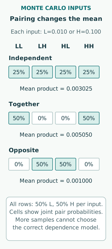
Let two uncertain inputs each take 0.010 or 0.100 with equal probability. In this original example their marginals are identical, with means 0.055. If sampled independently, their mean product is 0.055² = 0.003025. There are four equally likely input pairs, and direct enumeration gives the same result without simulation.

If the inputs always take the low state together and the high state together, their mean product is (0.010² + 0.100²)/2 = 0.005050. If they always take opposite states, the product is always 0.001000. The three models have identical marginal distributions and different joint distributions. More Monte Carlo samples would estimate each model more precisely without deciding which model is physically or epistemically justified.

Carry the units through the model

Suppose ν is fixed at an illustrative 0.20 per operating year and the two inputs are valid conditional probability quantities in the scenario model. Mean consequence frequencies are then 0.000605, 0.001010 and 0.000200 per operating year for the independent, together and opposite uncertainty models respectively. These are means of model outputs under the assigned parameter distributions.

They are not three observed accident rates, and their spread is not automatically a confidence interval. The example compares alternative dependency assumptions. If ν is also uncertain and related to the branch inputs, its joint relationship must be represented too. Multiplying separately reported means generally does not reproduce the mean of a nonlinear model with dependent inputs.

Distinguish output spread from sampling error

The spread of sampled consequence frequencies describes the uncertainty propagated from the input model. Monte Carlo sampling error describes how accurately a finite simulation estimates features of that distribution, such as its mean or a percentile. Increasing sample count can reduce numerical sampling error while leaving the underlying output spread essentially unchanged.

For independent identically distributed samples with finite variance, the standard deviation of a sample mean is the output standard deviation divided by the square root of sample count. If samples are correlated, that simple expression is not generally valid without accounting for the dependence. The uncertainty distribution and the numerical error of its estimated summary should be reported as different quantities.

See why rare events need special attention

The NIST binomial model gives a direct calculation for an independent event-counting simulation. Suppose the true event probability is an illustrative p = 0.0001 and N = 100,000 independent trials are simulated. The expected event count is Np = 10. The standard deviation of the estimated proportion is √[p(1 − p)/N], giving relative standard error approximately 31.62%.

With N = 10,000,000 trials, expected count is 1,000 and relative standard error is approximately 3.162%. A hundredfold increase in trials improves this measure tenfold under the assumptions. Observing zero events in one run would not establish zero probability. A visibly stable rounded display can also hide substantial relative uncertainty in a small probability.

Use targeted sampling only with the correct estimator

Primary research on importance sampling for unions of rare events addresses the difficulty of estimating rare-event probabilities efficiently. Methods that sample important regions more often can help, but the estimate must account for the changed sampling distribution. The fraction of failures in a deliberately biased sample is not the original event probability.

The choice and validation of an advanced estimator should match the event structure. It needs support over the relevant region and checks that its weights and uncertainty estimates behave as intended. A method that looks efficient on one test case may miss another important mode. For an educational risk study, a transparent exact benchmark and a simple verified estimator can be more informative than an unexplained impressive runtime.

Test convergence for the quantity you will use

A stable mean does not demonstrate that an extreme percentile or exceedance probability is accurately estimated. Choose the numerical quantity that supports the decision and assess precision for it. Independent repeat runs, growing sample sizes and analytically solvable cases can reveal problems that one fixed seed cannot. A seed is useful for reproducibility, not proof of correctness.

Input checks should confirm probability bounds, positive rates where required, units and the intended dependencies. Output checks should verify limiting cases and known identities. If an invalid sample is discarded, explain why and whether the rejection changes the intended distribution. Silently clipping impossible probabilities or repeatedly resampling inconvenient results changes the model rather than merely cleaning the simulation.

Report what simulation has and has not resolved

A reproducible record includes the model version, distributions and their evidence, joint-dependence assumptions, sample interpretation, estimator, random-number setup and convergence evidence. Show sensitivity to important modelling alternatives as well as the numerical result. This makes it possible to distinguish a software defect, insufficient sampling and a genuine disagreement about the underlying risk model.

Monte Carlo is a calculation method, not a source of physical knowledge. It can propagate what the model says with impressive precision while missing an unmodelled hazard or dependency completely. Its strongest use is to make uncertainty and nonlinear interactions visible, with enough numerical evidence to show that the reported summaries describe the stated model accurately.

Sources

• JCGM101:2008: Propagation of distributions using a Monte Carlo method · JCGM/BIPM · Source check date: 2026-10-07
• Binomial Distribution · NIST/SEMATECH · Source check date: 2026-10-07
• Importance sampling the union of rare events with an application to power systems analysis · Research authors via arXiv · Source check date: 2026-10-07