Knowledge / Risk analysis methods
Bayesian reliability updates: learning from sparse failure data
Use transparent prior and likelihood assumptions to update a demand-failure probability, inspect prior sensitivity and distinguish parameter uncertainty from future failures.
On this page
Sparse reliability data rarely support a confident conclusion on their own. Bayesian updating provides a formal way to combine an explicitly stated prior assessment with new observations. Its value is not that it creates information where none exists, but that it exposes how the starting assumptions and the data contribute to the result. For maritime equipment, the central questions remain whether the observations represent the intended service and whether the prior describes a genuinely relevant population.
Define the parameter before choosing a prior
The NIST Bayesian reliability overview distinguishes a prior, a likelihood for observed data and a posterior distribution. Let p denote the unknown probability that a specified protective function fails on one comparable demand. The function, starting condition and definition of a demand must be fixed before p has a useful meaning.
Assume demand outcomes are independent conditional on p and that the same p applies throughout the dataset. These are modelling assumptions, not consequences of using Bayes’ rule. A persistent hidden fault, changing operating conditions or several records from one shared disturbance can violate them. An update that ignores those features can be numerically exact for the wrong likelihood.
Use a conjugate model transparently
NISTIR 6129, section 3.4 presents beta–binomial updating. Although its application is software testing, the mathematical model can be stated independently. Here p is failure probability, rather than success probability. A Beta(a,b) prior combined with x failed demands out of n demands gives a Beta(a + x, b + n − x) posterior.
The posterior mean is (a + x)/(a + b + n). The positive parameters a and b determine both the prior mean a/(a + b) and its concentration. Their sum influences the weight of the prior relative to new observations, but need not represent literal historical test counts. Record how the prior was obtained instead of inventing a fictitious dataset to justify convenient parameters.
Calculate an original demand example
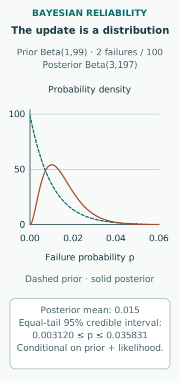
Suppose an explicitly illustrative prior is Beta(1,99), with mean 0.010. Observe two failed demands among 100 comparable demands, under the stated likelihood assumptions. The posterior is Beta(3,197), with mean 3/200 = 0.015. The raw observed fraction is 2/100 = 0.020; the posterior mean lies between that fraction and the prior mean.
The difference is not an error or an automatic improvement in truth. It is the result of giving the chosen prior substantial weight. If that prior was based on equipment in materially different service, the apparently moderate estimate can be misleading. Before using the result in a risk model, examine the prior population, failure definitions, test conditions and independence of the new records.
Report uncertainty rather than only the mean
For the Beta(3,197) posterior, the equal-tail 95% credible interval is approximately 0.003120 to 0.035831, obtained from the 2.5th and 97.5th percentiles. Under the specified prior and likelihood, the posterior assigns 95% probability to p lying within those bounds. This is a conditional model statement, not a claim that all relevant uncertainty has been captured.
The interval does not include uncertainty about whether the selected demands represent a different operating mode, whether failures were missed or whether the model omits a shared cause. A narrow posterior from a large but unrepresentative dataset can therefore be less useful than a wider assessment with the right boundary. Report those model and data limitations alongside the statistical interval.
Check how much the prior changes the conclusion
Keep the same two failures in 100 demands but use Beta(2,198), which has the same prior mean 0.010 and greater concentration. The posterior becomes Beta(4,296), with mean approximately 0.013333. Using a uniform Beta(1,1) prior instead gives Beta(3,99), with mean approximately 0.029412. The uniform prior is flat over p from zero to one; that does not make it neutral for every rare-failure question.
These alternatives are a sensitivity exercise, not a menu from which to select the most favourable answer. A defensible prior should be chosen and documented using relevant knowledge and the intended inference. If plausible priors lead to materially different decisions, the sensitivity is part of the result and may identify a need for better data or a more limited claim.
Interpret zero failures without declaring perfection
In a separate example, begin again with Beta(1,99) and observe no failures in 20 comparable demands. The posterior is Beta(1,119), with mean 1/120, approximately 0.008333. The mean decreases but does not become zero. The posterior probability that p exceeds 0.020 is (1 − 0.020)¹¹⁹, approximately 0.090345.
That tail probability is tied to this prior and dataset. It is not the same quantity as a frequentist confidence bound or the probability that a failure will occur on a particular future mission. The zero-failure observation can update the stated model while leaving considerable uncertainty. No-demand periods, incomplete logging and tests that omit the relevant failure mode should not be counted as successful representative demands.
Distinguish a parameter estimate from prediction
For the first Beta(3,197) posterior, the predictive probability of failure on the next comparable demand is the posterior mean 0.015. For ten future demands that are independent conditional on the same p, the probability of at least one failure is 1 − E[(1 − p)¹⁰]. Under this posterior it equals 1 minus the product of (197 + k)/(200 + k) for k from zero through nine, approximately 0.137410.
Substituting the mean first gives 1 − (1 − 0.015)¹⁰, approximately 0.140270, a different value. The exact predictive calculation averages over uncertainty in p; replacing p with one estimate removes that uncertainty before applying a nonlinear expression. Conditional independence given p also does not imply that the predictive outcomes are independent after p has been integrated out.
Keep time-based data in a compatible model
NIST’s gamma–exponential reliability discussion uses a different conjugate model for failure-rate information and accumulated operating time. Demand counts should not be added to operating hours, or beta parameters treated as gamma parameters, simply because both procedures are Bayesian. The likelihood determines which evidence updates which parameter.
Avoid counting the same historical observations twice, once in the prior and again in the new likelihood. Keep provenance at dataset level, including common fleet records and later revisions. When the equipment or operating regime changes materially, assess whether a hierarchical, time-varying or separate-population model is warranted. A more elaborate model should answer a real mismatch, not merely make a sparse dataset look sophisticated.
Carry the assumptions into the engineering decision
A useful update record identifies the parameter, prior rationale, likelihood, included and excluded observations, posterior summaries and sensitivity. The engineering model receiving the result must use the same demand definition and conditions. Posterior uncertainty can be propagated through that model, while scenario and consequence uncertainties remain separately visible.
Bayesian updating is a disciplined way to learn within a stated model. It does not certify equipment, supply missing failure mechanisms or guarantee that a fleet average applies to one ship. Its strongest contribution is a transparent account of what the new evidence changed, what the prior still influences and where the next useful observation would reduce uncertainty.
Sources
- Bayesian methodology for reliability evaluation · NIST/SEMATECH · Source check date: 2026-10-07
- NISTIR6129: Software Testing by Statistical Methods, 1998 · NIST · Source check date: 2026-10-07
- Models and assumptions for Bayesian reliability evaluation · NIST/SEMATECH · Source check date: 2026-10-07