Dependent event-tree branches: why conditional probabilities matter

Name the mechanism behind the dependency

IAEA’s published dependency guidance distinguishes functional, physical, human-interaction and component-failure dependencies. Used as a modelling reference, this helps ask what connects the two functions. A shared electrical supply differs from fire damaging separate cables, and both differ from two actions relying on one mistaken diagnosis. A single unexplained correlation coefficient would obscure those mechanisms.

For an illustrative shipboard arrangement, let protective functions A and B require one utility U. Their separate local hardware can fail while the utility remains available. The model below concerns availability at one defined demand under one specified initiating condition. It is not a continuous repair model, a generic equipment failure rate or a statement about any actual vessel design.

Define conditional local failures

Assume an invented probability 0.020 that U is unavailable at the demand. If U is unavailable, both functions fail. If U is available, local A failure has probability 0.030 and local B failure has probability 0.040; those two local events are assumed independent within the utility-available condition. These assumptions, including the deterministic loss of both functions with U, are part of the model.

Conditional independence is narrower than ordinary independence. It says that after the utility state is fixed as available, learning the local A outcome does not change the local B probability in this particular example. It does not say the complete function failures are independent when the utility state is unknown. Distinguishing the local event from the complete function is therefore essential when importing a number into the event tree.

Calculate the complete function probabilities

The total-probability framework in MIT’s conditioning lecture permits separate calculations for the utility states. Function A failure is 0.020 + 0.980 × 0.030 = 0.0494. Function B failure is 0.020 + 0.980 × 0.040 = 0.0592. Both probabilities already include the shared utility failure; neither is merely the local hardware input.

The joint failure probability is 0.020 + 0.980 × 0.030 × 0.040 = 0.021176. The first term covers utility unavailable; the second covers utility available and both local failures. Those alternatives are mutually exclusive. Multiplying the two complete marginal probabilities instead gives 0.0494 × 0.0592 = 0.00292448, far below the stated joint model. The smaller product has silently discarded their shared dependency.

Put the right number on each branch

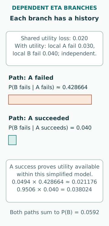
If the event tree tests complete A failure first, the following B-failure probability on that path must be P(B fails|A fails) = 0.021176/0.0494, approximately 0.428664. The value is much larger than the unconditional B-failure probability 0.0592. Observing A failure increases the inferred chance that the shared utility is unavailable; it does not physically damage B merely by being observed.

On the A-success path, the utility must be available under the assumptions. The probability that B fails there is 0.040, its conditional local value. Applying the same B probability to both paths would contradict this model. A practical worksheet can record the path state beside the branch input, making it clear why visually identical B headings carry different values.

Check all four terminal sequences

The four sequence probabilities are: both fail 0.021176; A fails and B succeeds 0.028224; A succeeds and B fails 0.038024; both succeed 0.912576. Their sum is one. Adding the first two returns A’s marginal 0.0494; adding the first and third returns B’s marginal 0.0592. These checks test different aspects of the bookkeeping.

A tree can satisfy the sum-to-one test while using the wrong dependency. Independent branch probabilities also create a normalized tree, but they create a different joint distribution. Compare the implied joint events with the physical model and source inputs. Numerical normalization checks the total assigned probability mass. It does not by itself prove that the events are disjoint, that they exhaust the selected sample space, or that the model includes every relevant failure mechanism. MIT’s sum rule requires disjoint events as a premise.

Condition on the initiator itself

The assumed 0.020 utility unavailability is valid only for the defined initiating condition. If the initiating event is loss of that very utility, then its conditional unavailability is one, and both dependent functions fail in this simple no-alternate-support model. Retaining 0.020 on that tree would give credit to support that the initiator has explicitly removed.

Another initiator might leave the utility mostly unaffected, damage it with a conditional probability, or change the duration for which it is required. These are different models. Record whether the initiator frequency already represents a support failure and whether the support event reappears inside a heading. Otherwise the same event can be counted twice, omitted, or assigned a probability inappropriate to the condition being analysed.

Convert to frequency on the stated exposure basis

NRC’s PRA explanation connects event-tree sequences with fault-tree analyses of their functional headings. In an original example, suppose the defined initiator has frequency 0.40 per operating year and the preceding demand model applies at every such occurrence. The frequency of the both-fail sequence is 0.40 × 0.021176 = 0.0084704 per operating year.

That number is an expected occurrence rate for the defined sequence, not automatically the probability of a loss in one year. Consequences after both failures still require a physical endpoint model. If the initiator population mixes different modes or support conditions, use compatible conditional models and exposures rather than multiplying one fleet-wide frequency by a convenient average branch probability.

Test what a proposed change actually changes

For an independent sensitivity exercise, reduce only the assumed utility unavailability to 0.005 while keeping the two conditional local probabilities at 0.030 and 0.040. The joint failure becomes 0.005 + 0.995 × 0.030 × 0.040 = 0.006194. This is a change in one model parameter, not evidence that a particular maintenance action will achieve it.

Adding a second supply cannot be represented by that reduction without investigating switching, common distribution, control power, capacity and exposure to the same hazard. Conversely, improving only A’s local hardware leaves the common utility contribution intact. A dependency model helps identify what evidence a proposed improvement must provide, rather than promising risk reduction from the number of installed components.

Preserve the boundary of the probability claim

The analysis should identify every basic event consistently, record conditional datasets and distinguish measured inputs from assumed ones. A shared support failure explicitly represented in the logic should not also be hidden inside a second empirical function probability unless their overlap is reconciled. The same discipline applies to human actions and environmental damage.

The worked model is deliberately small so that its conditional arithmetic can be checked by hand. Real equipment may retain partial capability, operate on stored energy, recover before the deadline or fail through additional shared causes. Those features belong in the state and success criteria when they matter. Correct multiplication follows a defensible model; it cannot compensate for a missing mechanism.

Sources

• SSG-3 (Rev. 1): Analysis of Dependent Failures · IAEA · Source check date: 2026-10-06
• Introduction to Probability, Lecture 2: Conditioning and Bayes’ Rule, 2018 · MIT OpenCourseWare · Source check date: 2026-10-07
• Probabilistic Risk Assessment · US NRC · Source check date: 2026-10-06
• Mathematics for Computer Science, Lecture 19: Conditional Probability, 2024 · MIT OpenCourseWare · Source check date: 2026-10-07