Failure rate and demand probability: choosing the right reliability quantity

Use units to identify the question

A rate has an inverse-time unit, such as h⁻¹, when time is its exposure. A probability is dimensionless and lies between zero and one. A probability per demand describes an outcome conditional on a specified demand; the word demand is part of the experiment, not a time unit. An expected count is also dimensionless, but unlike a probability it can exceed one.

The units alone do not identify every difference. A lifetime hazard rate and a repairable system’s rate of occurrence of failures can both be written h⁻¹ while referring to different conditioning. Retain the event definition, repair treatment and population beside the number. A column headed reliability without those details invites the wrong conversion even when every entry has been copied accurately.

Distinguish first-failure hazard from repeated failures

The NIST exponential model describes a lifetime distribution with constant hazard. Hazard concerns the instantaneous failure tendency conditional on survival to the current time. For a nonrepairable item, the lifetime ends at its first failure. The model is an assumption about that population and exposure, not a universal property of machinery.

The NIST homogeneous Poisson process instead models repeated failure occurrences at a constant rate. It can be relevant to a repairable-system counting process under its assumptions. The same numerical parameter can appear in exponential waiting times and Poisson counts, but that mathematical relationship does not permit silently treating a damaged, ageing or imperfectly repaired system as an unchanged process.

Convert a constant hazard with the mission time

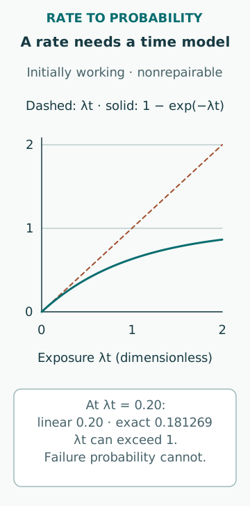
Assume an illustrative constant hazard λ = 0.000200 h⁻¹ for an initially functioning nonrepairable item. Over t = 10 h, first-failure probability is 1 − exp(−λt) = 1 − exp(−0.002), approximately 0.001998. The small-exposure approximation λt gives 0.002. The rate alone did not define the mission probability; time and the model were necessary.

For 1,000 h under the same assumption, λt = 0.20 but the exact first-failure probability is approximately 0.181269. The difference is now material for many uses. The linear approximation can eventually exceed one, which reveals why it cannot be a probability formula for arbitrary exposure. Always specify whether a displayed value is exact under the model or an approximation with a checked range.

Do not confuse an expected count with at least one failure

In a separate homogeneous Poisson counting example with rate 0.000200 h⁻¹ over 1,000 h, the expected number of occurrences is 0.20. The probability of at least one occurrence is 1 − exp(−0.20), approximately 0.181269. The numerical probability matches the exponential first-arrival result because the models are linked in this specific way.

Expected count 0.20 does not mean exactly one failure occurs with probability 0.20; the counting model also permits two or more. Nor does a rate estimate promise regularly spaced failures every 5,000 h. The inverse rate is a mean interval under the stated process. A calendar-based maintenance or operational claim needs additional failure-mechanism and exposure evidence.

Define the demand before estimating its failure probability

The NIST binomial distribution models counts from independent trials with a common outcome probability. In an original demand example, let failure probability be p = 0.002 for each of 200 comparable independent demands. Expected failed demands are np = 0.4. The probability of at least one failed demand is 1 − (1 − 0.002)²⁰⁰, approximately 0.329948.

The independence and common-probability assumptions matter. If a hidden fault persists through several demands until repaired, successive outcomes can be linked. If difficult demands occur in a different operating mode, one common p may be inappropriate. A start command, an observed successful start and a complete mission are also different endpoints. The data and calculation must use the same definition.

Relate demand frequency to failed-demand frequency carefully

Suppose demands occur at a mean rate of 0.10 per operating hour, and each demand has failure probability 0.002 under conditions independent of the demand-arrival process and consistent with the model. The expected failed-demand rate is 0.10 × 0.002 = 0.000200 per operating hour. Under stronger independent Poisson-thinning assumptions, the failed-demand count is itself a Poisson process.

This resulting occurrence rate is not automatically the equipment’s physical failure hazard. It combines how often a challenge arrives with the chance of an unsuccessful response. Reducing demand frequency can reduce failed responses per year without changing equipment capability on a demand. Conversely, increased exposure can raise the annual count even if the response probability improves.

Keep operating, standby and calendar exposures separate

A device can accrue degradation while running, while idle or through repeated cycles. The relevant denominator depends on the mechanism. A running-hour failure estimate cannot be applied to calendar hours merely because both use the word hour. A demand-based estimate cannot be converted to an hourly equipment rate without a demand model and clear interpretation.

A mixed mission may require separate states, with different hazards, opportunities for detection and repair, or a transition event. Preserve those distinctions before aggregation. Averaging data from continuously running pumps and rarely demanded standby pumps can hide differences in failure detection and exposure. A larger combined dataset is not necessarily a more relevant dataset.

Check the boundary of the source data

A component record may include failure to start but omit failure to continue, external power loss or maintenance unavailability. Another source may include all of them in a complete-function probability. Before combining values, identify their boundaries, time basis, failure modes, censoring and treatment of repair. Otherwise an event can be omitted or counted twice.

Zero observed failures also needs its exposure. Zero in a short observation is not evidence of a zero rate; zero failed demands with no real demands is not a measured zero failure probability. Retain uncertainty and distinguish a statistical estimate from a design assumption. The number of significant digits should not imply confidence that the dataset and model do not provide.

Choose the input the model actually asks for

For each event-tree branch or fault-tree basic event, write the needed quantity before choosing a source. Is it probability of failure at a demand, failure during a defined running interval, known unavailability in the present configuration or an occurrence frequency? Then document the conversion, if any, and its assumptions. This makes the calculation reproducible and exposes incompatible inputs early.

Rates and probabilities are connected by models, not by interchangeable labels. The right quantity keeps the event, time, demand and repair meaning intact. That discipline often matters more than refining a decimal place, because a precisely calculated result from the wrong reliability quantity still answers the wrong question.

Sources

• Exponential lifetime model · NIST/SEMATECH · Source check date: 2026-10-07
• Homogeneous Poisson Process · NIST/SEMATECH · Source check date: 2026-10-07
• Binomial Distribution · NIST/SEMATECH · Source check date: 2026-10-07