Load-sharing reliability: changing damage rates after the first failure

Define what one surviving unit must accomplish

Consider two identical generic units that are active from the start and share a constant total demand equally. Either unit is physically capable of carrying the full demand alone, so the system remains functional after the first unit failure. This capability condition is essential. If a single unit cannot meet the required output, the first failure already ends the mission and the proposed redundancy model is wrong.

Assume instantaneous load redistribution, no transfer failure and no repair during a 2000 h mission. The numerical example uses operating hours. A higher load is represented by a higher failure hazard, not by a measured crack-growth law. Every rate is fictional. Separating these assumptions makes the simple example useful without implying that all real load-sharing mechanisms are memoryless or respond instantly.

Describe the states and the two transition rates

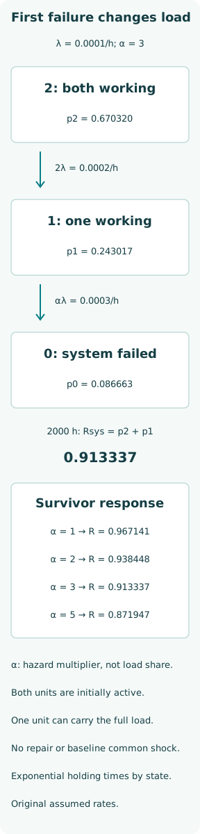
Let state 2 mean both units work, state 1 mean one works, and state 0 mean system failure. While both work, each has hazard λ = 0.0001/h, so the total transition rate from state 2 to state 1 is a = 2λ = 0.0002/h. After the first failure, the remaining unit has hazard b = αλ, with α = 3, hence b = 0.0003/h.

Load-sharing models let a component’s hazard change with the operating status of other components. The multiplier here is a hazard ratio, not the fraction of total load. Moving from half to full load does not automatically imply that hazard doubles. The load-to-hazard response must be measured, derived from a suitable physical model or explicitly treated as an uncertain assumption.

Build the mission probability from state occupancy

Write p2(t), p1(t) and p0(t) for the state probabilities, starting from p2(0) = 1 and the other two equal to zero. The forward equations are p2′ = −a p2, p1′ = a p2 − b p1 and p0′ = b p1. Their sum has zero derivative, so probability is conserved. The failed state is absorbing because no repair is allowed within this mission.

The first equation gives p2(t) = exp(−at). The one-survivor probability is p1(t) = ∫₀ᵗ a exp(−au) exp[−b(t − u)] du. This integrates every possible first-failure time u and the chance that the remaining unit lasts to the horizon. For b ≠ a, p1 = a[exp(−at) − exp(−bt)]/(b − a). System reliability is p2 + p1, not p2 alone.

Compute the original two-unit result

At 2000 h with α = 3, p2 = 0.670320 and p1 = 0.243017. Thus Rsys = 0.913337 and system failure probability is 0.086663, rounded to six decimals. The exact values sum to unity across the three states. The one-survivor probability describes a system that is currently functional but has used up its unit redundancy and now faces the higher hazard.

The time to system failure is the sum of an exponential holding time with rate a and a subsequent one with rate b under this model. Its mean is 1/a + 1/b = 8333.333333 h. This mean does not replace the mission probability: two architectures can have similar mean lives yet different survival at the specified mission horizon. Nor is it a repaired-system mean time between failures.

Use the unchanged-hazard limit as a diagnostic

If α = 1, losing the partner leaves the survivor’s hazard unchanged. The state solution reduces to Rsys(t) = 2 exp(−λt) − exp(−2λt), which is the ordinary independent active-parallel result. NIST’s parallel model requires independent component operation. At 2000 h it gives reliability 0.967141 and failure probability 0.032859, considerably below the failure probability under the assumed load transfer.

For α = 2, b equals a and the displayed quotient has a removable zero-over-zero form. Use its limit p1 = at exp(−at), giving reliability 0.938448. With α = 5, reliability is 0.871947. These sensitivity cases hold the initial shared-load hazard fixed. They show how the unverified survivor response can dominate the benefit assigned to an extra active unit.

Retain the time of the first failure

If the first failure occurs at 500 h, the survivor must last another 1500 h and its conditional survival is exp(−0.0003 × 1500) = 0.637628. If the first failure occurs at 1500 h, only 500 h remain and survival is 0.860708. The distinction follows from time spent under the higher load, even though the exponential model has no additional memory of earlier shared-load service.

It is therefore incorrect to assign every mission the full-load hazard for its entire duration or to apply the shared-load hazard after the partner fails. The convolution over first-failure times handles the changing exposure. With nonexponential hazards, the survivor may also retain damage accumulated before transfer, so the post-transfer distribution can depend on the full load history as well as the remaining mission duration.

Separate load redistribution from common-cause failure

In the baseline model, one unit fails first and changes the survivor’s subsequent hazard. There is no positive probability of exactly simultaneous failures from a shared shock. A common-cause event instead can disable both units directly, or alter their conditions through another shared mechanism. These are different pathways; labeling every dependent failure “common cause” can hide which engineering action would reduce it.

As a separate extension, assume independent fatal shocks with rate γ = 0.00002/h that kill the system from either functioning state. Then reliability becomes exp(−γt) times the baseline load-sharing reliability, yielding 0.877524 at 2000 h. This factorization requires the shock process to be independent and unaffected by the unit state. It cannot be used if the same load transfer already accounts for the shock pathway.

Distinguish two active units from a cold spare

A standby model activates a spare after the operating unit fails. Here both units operate and contribute before the first failure. Their pre-transfer exposure and the first-failure rate are consequently different from a system with one dormant spare. The spare’s dormant aging, activation reliability and switching time may also need explicit states, even when its nominal operating failure law matches the active unit’s.

A fair architectural comparison must use hazards appropriate to each unit’s actual load and environment. Using a half-load hazard for the initially full-load active unit in a standby calculation gives an artificial advantage. Likewise, a load-sharing design that sheds demand after a failure changes the success criterion unless reduced output is explicitly acceptable. Define the required function before comparing curves across these architectures.

Choose a richer model when history matters

The state count is sufficient here because all holding times are exponential and the units are identical. Real degradation can depend on cumulative cycles, stress amplitude, time since transfer or which specific unit remains. In those cases, add age or damage states, distinguish unit identities, use a semi-Markov formulation or simulate the specified degradation law. A change in hazard is a useful approximation, not a complete material-damage model.

Load-sharing inference distinguishes successive failure stages and their parameters. Record which units worked, their loads, transfer times and censoring. Total fleet hours alone mix shared-load and survivor exposure. Few observed survivor failures can leave α poorly estimated even when the initial hazard is precise. Report that uncertainty and check predictions after transfer, where the model’s key claim is actually being used.

Connect sensitivity to a concrete design decision

Possible actions include reducing post-failure demand, improving full-load thermal capacity, shortening the permitted degraded-operation interval or adding an independently supported spare. Each changes different model elements. Faster repair can help a real maintained system, but it needs return transitions and repair-time assumptions; it cannot be credited by simply replacing the absorbing failed state’s probability with an availability value.

For the present case, verify probability conservation, the α = 1 independent limit, the α = 2 equal-rate limit and decreasing reliability as survivor hazard increases. Then check that one unit can still deliver the required service. Those numerical and functional checks reveal whether the assigned redundancy benefit follows from a defensible load-sharing mechanism rather than from drawing two boxes in parallel.

Sources

1. Kvam and Peña — Estimating Load-Sharing Properties in a Dynamic Reliability System.
2. NIST/SEMATECH — Parallel or redundant model.
3. NIST/SEMATECH — Standby model.
4. Reliability demonstration test for load-sharing systems with exponential and Weibull components.