Knowledge / Risk analysis methods
Maintainability: mean repair time, delays and probability of timely restoration
Compare two restoration distributions with the same mean but different deadline and tail performance, while separating active work from administrative and logistic delay.
On this page
An average restoration time can hide two very different support arrangements. One may usually finish quickly but occasionally wait much longer for a part; another may be slower in ordinary cases yet avoid a long tail. This original example keeps their mean equal and asks what each arrangement can actually deliver before a defined deadline.
Define restoration before measuring its duration
Start the clock at detection of the specified functional loss and stop it after the function has been restored and verified against its acceptance criteria. Call the resulting elapsed duration D, measured in hours. If the record instead starts when a technician arrives, it measures another interval and cannot silently replace the full restoration clock in an operational decision.
NASA’s maintainability definition ties restoration to specified personnel, procedures, resources and conditions. State those conditions for the equipment and support arrangement being compared. Restoring a component, transferring service to a standby unit and returning the original system to unrestricted operation may have different endpoints. The duration distribution belongs to one endpoint and one population of tasks.
Separate active work from waiting without losing elapsed time
In the fictional case, active maintenance comprises 0.5 h diagnosis, 0.25 h access preparation, 1 h hands-on work and 0.25 h verification: 2 h in total. Administrative delay is another 0.5 h. Logistic delay L supplies the remaining sequential interval, so D = 2.5 h + L. These numbers are assumed work stages, not stopwatch observations.
NASA’s maintenance metrics distinguish active maintenance from logistic and administrative delay, and distinguish means from percentiles. Preserve those definitions in the dataset rather than relying on the ambiguous abbreviation MTTR. In a real task, stages may overlap; then elapsed time follows a dependency schedule, not the sum of all recorded labor hours. The addition here is valid because sequential stages are explicitly assumed.
Construct two distributions with the same mean
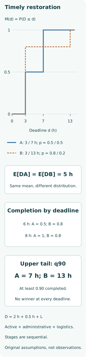
Arrangement A has logistic delay 0.5 h with probability 0.5 and 4.5 h with probability 0.5. Its total restoration duration is therefore 3 h or 7 h with equal probability. Arrangement B has logistic delay 0.5 h with probability 0.8 and 10.5 h with probability 0.2, giving total durations 3 h or 13 h.
Both means are 5 h: E[DA] = 0.5 × 3 + 0.5 × 7, while E[DB] = 0.8 × 3 + 0.2 × 13. Their active-maintenance mean is also identical at 2 h. The discrete values make the calculation auditable; real durations would vary within each support state. The example does not claim that repair work literally has only two possible completion times.
Ask for completion probability at the actual deadline
Define M(d) = P(D ≤ d), including completion exactly at d. At a 6 h deadline, MA = 0.5 and MB = 0.8, so B is more likely to restore in time. At an 8 h deadline, MA = 1 and MB = 0.8, so A is better. Neither arrangement is uniformly preferable across all deadlines despite the equal means.
A single statement that “B is faster” would miss the crossing of the two completion distributions. Select the deadline from the service requirement, available alternative support or tolerated outage, not after inspecting which arrangement wins. The deadline does not make unsafe work permissible; it is a criterion for evaluating the support capability under the stated safe task procedure.
Read the upper quantile as a tail requirement
Define q90 as the smallest duration at which cumulative completion probability reaches at least 0.90. In this discrete example q90 is 7 h for A and 13 h for B. A high proportion of short B cases does not remove its longer upper tail. The stated quantile convention also makes behavior at the probability jumps unambiguous.
A percentile is not a worst-case guarantee: a requirement framed at that percentile accepts that some cases may take longer. Actual tail estimation needs enough relevant observations and uncertainty assessment. A sparse dataset with no rare logistics delay observed can make the apparent tail too short. The support-state probabilities in this example are supplied assumptions and have no sampling confidence attached.
Measure how late a missed restoration is
Deadline success treats all late cases alike. Add expected excess duration E[(D − d)₊], where the positive-part symbol means zero when restoration is on time. At d = 6 h, A has 0.5 h expected excess and B has 1.4 h. B wins on timely-completion probability at that deadline but loses on this measure of average time beyond it.
At d = 8 h, expected excess is zero for A and 1 h for B. These are unconditional expected excess hours across all cases, not the average lateness only among late cases. If a case is still unrestored at 6 h, the remaining time in the stipulated discrete model is 1 h for A and 7 h for B. Observing noncompletion changes which support state is possible.
Do not invent an exponential repair rate from the mean
Taking μ = 1/5 h⁻¹ from the common mean and assuming an exponential restoration law would give M(6) = 0.698806, M(8) = 0.798103 and q90 = 11.512925 h. These values match neither original distribution. The exponential model supplies a constant hazard; adopting it adds a distributional assumption, not merely a convenient unit conversion.
Its memoryless remaining-time property is especially different from the known discrete support states. A mean is useful for some long-run calculations, but it cannot determine a deadline probability without a distribution. If a Markov availability model uses a single repair transition rate, check whether its holding-time assumption is adequate for the decision and whether logistic delay belongs in that state definition.
Keep unfinished jobs in the evidence
A job still open when data collection ends has a duration known only to exceed its elapsed time. Censoring methods preserve that information rather than replacing it with a completed duration. Dropping open jobs preferentially removes long cases. Recording the report date as completion instead compresses the tail and can overstate timely restoration.
Track failure detection, authorization, parts request and arrival, access, active work and functional acceptance timestamps. Keep reasons for task suspension, unsuccessful repair and repeat work. A change in spares location, route, crew or vendor support may create a different population. Pooling those cases without their context can manufacture a mean that describes neither the old support system nor the new one.
Target the delay that changes the chosen service measure
For B, reducing its slow logistic state from 10.5 h to 5.5 h changes the slow total from 13 h to 8 h. Its mean drops to 4 h, and its 8 h completion probability becomes 1 while its 6 h completion probability stays 0.8. This hypothetical intervention directly addresses the long-delay state; it is not evidence that purchasing a spare will achieve the assumed reduction.
By contrast, reducing active work slightly can improve the mean without moving any probability mass across the relevant deadline. Use task and logistics evidence to identify which stage controls the desired quantile or completion probability. Include transport permissions, compatible parts, verification resources and concurrent demand when those conditions determine whether a proposed support change is actually available to the failed equipment.
Use means for their proper purpose and retain the tail
Suppose an ideal alternating-renewal system has mean uptime 100 h and either restoration distribution, with independent identically distributed regenerative cycles and no other outages. Both give the same long-run availability, 100/(100 + 5) = 0.952381. The equality is compatible with their different deadline performance; long-run time fraction and timely return after one loss are distinct service measures.
A useful maintainability comparison therefore reports the clock, active work, delays, mean, selected deadline probabilities and an appropriate tail measure. Add uncertainty and the operational conditions supporting each estimate. In this example, the equal mean is the beginning of the comparison. The decision depends on when service must return and what happens if the less frequent long outage occurs.