Mission time and risk aggregation: rates, probabilities and changing exposure

Define the clock and failure endpoint

The relevant clock may be operating time, time in a particular mode or calendar age. A mission can include running, standby and transitions, each with different failure opportunities. Define the functional endpoint and whether the calculation stops at its first occurrence or counts repeated occurrences after restoration. These choices determine the mathematical model.

A propulsion-related mission might be divided into phases for a bounded reliability study, but the phase names alone do not define hazard values. The data must correspond to the equipment state, duty and failure definition in each phase. A failure rate measured over mixed fleet service cannot automatically be assigned to one demanding phase merely because it is the only available number.

Integrate hazard rather than add probabilities blindly

The NIST hazard-rate discussion relates a nonrepairable lifetime’s survival to cumulative hazard H(t), the integral of the conditional hazard over time. Under that model, first-failure probability is F(t) = 1 − exp[−H(t)]. For piecewise constant hazard, H is the sum of each phase’s hazard multiplied by its duration.

The quantities added are cumulative-hazard contributions, not independent phase-failure probabilities. Each hazard is conditional on survival into the phase and appropriate to the state being modelled. The resulting probability remains between zero and one. Simply adding phase probabilities counts some hypothetical combinations inconsistently unless the necessary approximation and its error are established.

Calculate a two-phase mission

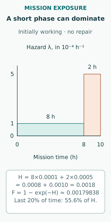
Consider an initially functioning, nonrepairable item with an invented hazard 0.000100 h⁻¹ during an 8 h first phase and 0.000500 h⁻¹ during a 2 h second phase. Assume these hazards depend only on the assigned phase and remain valid conditional on survival. Cumulative hazard is 0.000100 × 8 + 0.000500 × 2 = 0.001800.

Mission first-failure probability is 1 − exp(−0.001800), approximately 0.001798381. The time-weighted average hazard is 0.001800/10 = 0.000180 h⁻¹ and gives the same result over the same 10 h under this model. Taking the unweighted average of the two hazard values gives 0.000300 h⁻¹ and cumulative hazard 0.003, answering a different exposure question.

Understand what reordering phases assumes

In the deliberately simple example, exchanging the order of the two fixed phase exposures leaves the integrated hazard unchanged. That follows because the assigned hazards have no memory, ageing interaction or transition penalty beyond the stated phase. It is a mathematical property of this model, not a general statement that the order of ship operations is irrelevant.

If a hot phase changes the condition entering the next phase, a transition can induce failure, or an earlier impairment removes redundancy later, the hazards or states cannot be kept unchanged after reordering. A state-transition or degradation model may then be necessary. The mission model should represent the effect that makes order important instead of hiding it inside a generic average rate.

Distinguish repeated missions from continuous survival

The NIST binomial model supports a separate repeated-trial calculation. Suppose 20 missions each start in the same relevant condition and their failure outcomes are independent with the previous mission probability p = 1 − exp(−0.001800). Expected failed missions are 20p, approximately 0.035968. The probability of at least one failed mission is 1 − (1 − p)²⁰, approximately 0.035360.

The latter also equals 1 − exp(−0.036) under these particular inputs. That equality does not prove that the physical assumptions for repeating missions are met. A hidden fault persisting between missions, incomplete restoration or a shared environmental state can create dependence. State explicitly what establishes the repeated starting condition; merely beginning a new voyage record does not reset the equipment.

Use occurrence-rate models for repeated events when appropriate

NIST’s non-homogeneous Poisson-process discussion describes a time-varying occurrence-rate model for repairable-system events. Such a counting process is distinct from a nonrepairable first-failure lifetime even though both can involve an integral over time. The interpretation of the integrated quantity must stay with the model.

For a counting process with a specified intensity, the integral gives expected occurrences over the interval. Under a Poisson model, one minus the exponential of its negative gives the probability of one or more occurrences. If repair changes future behaviour, events cluster or the intensity depends on an unobserved state, a simple deterministic-intensity model may be inadequate. The same formula shape does not establish the same physical process.

Preserve uncertainty when converting to probability

In an original uncertainty example, suppose cumulative hazard H is either 0 or 0.020 with equal probability. Its mean is 0.010. Averaging the conditional failure probabilities gives [0 + 1 − exp(−0.020)]/2, approximately 0.009900663. Converting only the mean gives 1 − exp(−0.010), approximately 0.009950166. The values differ because the conversion is nonlinear.

Here the two states represent an explicitly assigned uncertainty distribution, not observed equal-frequency operating phases. For uncertain rates or durations, preserve their relationship before converting. A long exposure may occur precisely when hazard is elevated. Independently averaging the two inputs can remove that association and change the expected consequence. A sensitivity range and a probabilistic uncertainty model should also be labelled differently.

Connect mission exposure to calendar reporting carefully

A per-mission probability, expected failed missions per year and probability of at least one annual failure are different outputs. Converting requires the number and type of missions, their starting states and their dependence. Calendar downtime, inactive periods and maintenance can matter even when the operating-time model assigns no running exposure to them.

If mission duration is itself random, applying the model at the mean duration is generally not equivalent to averaging the mission probabilities. If failures shorten the observed mission, using only completed-mission durations can bias the exposure record. Keep the observation rules, censored durations and population definition visible when moving from service records to a mission model.

Report the aggregation with its assumptions

A useful result identifies the endpoint, time basis, phase durations, hazards or occurrence intensities, transitions, repair treatment and dependence assumptions. Show phase contributions and the exact conversion used, with a check on any small-probability approximation. This lets a reviewer see whether one short but demanding phase dominates the result.

Mission aggregation should preserve the engineering story as it reduces the data to a number. It can support comparisons of defined operating profiles and identify where better evidence matters. It cannot turn an unmatched failure rate into a vessel-specific prediction or establish an acceptable operating duration without the relevant physical, operational and regulatory basis.

Sources

• Failure (or hazard) rate · NIST/SEMATECH · Source check date: 2026-10-07
• Binomial Distribution · NIST/SEMATECH · Source check date: 2026-10-07
• Non-Homogeneous Poisson Process – power law · NIST/SEMATECH · Source check date: 2026-10-07