Knowledge / Risk analysis methods
Multi-unit PSA: shared events, simultaneous damage and limited response resources
A joint two-asset example separates expected damage count from any-damage and simultaneous-damage probabilities while enforcing one shared response resource.
On this page
Adding asset-level damage probabilities does not give the probability that a site has any damage. Shared hazards and limited response resources make the distinction operationally important. This original example follows one common event, preserves the joint demand states and allocates a finite resource before calculating three different damage measures.
Choose a site event and a joint endpoint
Consider two generic assets, A and B, exposed to a common disruptive event H with frequency 0.02 per site-year. Damage means that an asset fails its specified service criterion during the bounded event mission. The event can demand mitigation at neither asset, one asset or both. Here simultaneous damage means both assets meet the damage criterion within the same event mission, not necessarily at identical onset times. There are no nuclear systems, human casualty outcomes or acceptance thresholds in this example.
IAEA’s multi-unit PSA report distinguishes site events from sums of unit-specific frequencies. The same accounting issue arises here: damage to both assets is one site event but two damaged assets. Define whether the result will count events, count damaged assets, or describe concurrent damage before assembling the model; those quantities are not interchangeable summaries of “site risk.”
Preserve the four demand states
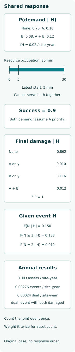
Conditional on H, stipulate demand probabilities of 0.70 for neither asset, 0.10 for A only, 0.08 for B only and 0.12 for both. These mutually exclusive states sum to unity. Their joint structure is supplied directly; it is not inferred by multiplying marginal demands. The common event has already occurred at this point, so its frequency is not inserted again inside each conditional probability.
A demanded asset will be damaged unless its mitigation succeeds. An undemanded asset remains undamaged in this deliberately simple model. This separation between demand and final damage matters: effective mitigation can move probability from a demand state to a different damage state. A model that labels the initial demand table as the final damage table would discard the response resource entirely.
Represent one resource with one simultaneous capacity
Assume one portable resource can serve either asset, but must remain with the selected asset for the entire 30 min mission. Effective mitigation must start within 5 min of the common demand. Both demands arrive together. The resource therefore cannot complete one mission and then start the other in time. These invented timing rules make the capacity constraint explicit without specifying real pump performance.
When only one asset demands help, allocate the resource there. When both demand help, stipulate A priority solely to define this toy policy. Let an allocated resource succeed with probability 0.9, conditional on any demand state in which it is allocated. The other demanded asset receives no resource and is damaged. This priority is an analysis input, not an emergency-response recommendation.
Enumerate the final damage distribution
For the A-only demand state, successful mitigation contributes 0.09 to no damage and failure contributes 0.01 to A-only damage. For the B-only state, the corresponding contributions are 0.072 and 0.008. When both demand help, resource success contributes 0.108 to B-only damage; resource failure contributes 0.012 to damage of both. Add the original no-demand probability to the no-damage result.
| A damaged | B damaged | Probability |
|---|---|---|
| 0 | 0 | 0.862 |
| 1 | 0 | 0.010 |
| 0 | 1 | 0.116 |
| 1 | 1 | 0.012 |
The final no-damage probability is 0.862. A-only damage is 0.010, B-only damage is 0.116, and both damage is 0.012. The four outcomes still sum to unity. The large B-only term is a transparent consequence of the stipulated resource allocation, not evidence that asset B has intrinsically less reliable equipment. Changing the policy would require rebuilding the joint outcomes.
Calculate the three distinct damage measures
Let N be the number of damaged assets in this event. The expected count is E[N | H] = 0.010 + 0.116 + 2 × 0.012 = 0.150 damaged assets per event. The probability of any damage is P(N ≥ 1 | H) = 0.010 + 0.116 + 0.012 = 0.138. The probability of simultaneous damage is P(N = 2 | H) = 0.012.
The marginal damage probabilities are P(A | H) = 0.022 and P(B | H) = 0.128. Their sum equals the expected count, regardless of dependence. Inclusion–exclusion gives any damage by subtracting the joint term once. Multiplying the marginals instead would give 0.002816 for both damage, which is incorrect here. The joint table, rather than a convenient independence assumption, determines the intersection.
Attach annual units to the correct quantity
Multiplying the conditional expected count by the event frequency gives 0.003 damaged assets per site-year. Multiplying the any-damage probability gives 0.00276 damaging site events per year. Multiplying the simultaneous-damage probability gives 0.00024 events with both assets damaged per year. These totals refer only to the specified common-event family; other initiating events are not included.
The first result can exceed the second because one event can damage more than one asset. None of these frequencies is automatically an annual probability of at least one occurrence. That conversion needs an event-counting model and a clear treatment of repair, repeated exposure and the availability of assets after earlier damage. Keep the conditional event calculation separate from that additional temporal question.
Compare genuinely separate response capacity
For comparison, stipulate two resources, each with its own simultaneously available support, and independent success probability 0.9 when required. In the both-demand state, both succeed with probability 0.81, exactly one succeeds with probability 0.18, and neither succeeds with probability 0.01. This is a new resource model, not a second credit applied to the unchanged single-resource arrangement.
The resulting final probabilities are 0.9592 for no damage, 0.0208 for A-only damage, 0.0188 for B-only damage and 0.0012 for both. Hence expected damaged count is 0.042 and any-damage probability is 0.0408. Annual results become 0.00084 damaged assets, 0.000816 any-damage events and 0.000024 both-damage events per site-year. Independence of the added support is essential to this comparison.
Do not spend the same resource twice
IAEA’s revised guide calls for explicit shared-resource availability and usage priorities in multi-unit models. In this generic example, applying the single-asset mitigation success separately to both assets would secretly assume the two-resource alternative. A second line in a fault tree does not create another portable device, crew, connection point or usable access route when demands occur together.
Resource capacity also has a time dimension. A kit that is reusable later may still be unavailable within the second asset’s required response window. A larger model should retain mobilisation, travel, access, installation, occupation and release times, including which tasks can overlap. Nominal equipment count is insufficient when the bottleneck is a shared crew or hazard-damaged route rather than the device itself.
Keep common-event and response dependencies separate
The initial demand table captures which assets are challenged together by H. The resource model determines which of those demands can be mitigated. These are distinct sources of dependence. Even with independent device performance, one shared allocation can couple final outcomes. Conversely, two physically separate resources can remain dependent through a common power supply, access restriction or team that must perform both actions.
If response success depends on event severity, condition it on the relevant hazard state before averaging. Do not combine a severe-event demand distribution with routine deployment success data without checking applicability. Likewise, an asset under maintenance may change both its vulnerability and resource demand. The site model must describe the joint configuration that exists when the event occurs, rather than stitching together incompatible best cases.
Verify the joint model and report its limits
Audit probability conservation at the demand split and at every response split. Independently enumerate resource allocations and final outcomes; verify that no scenario assigns the single resource to two simultaneous full-duration missions. Check that expected count equals the sum of marginal damage probabilities and that any-damage probability counts the joint outcome only once. These identities test different failure modes in the calculation.
Report the joint table, all three metrics, resource assumptions and conditional event frequency together. The example does not optimise emergency priorities or establish a real site’s resilience. Its useful result is a disciplined distinction: expected damaged-unit count, the chance of any damage and the chance of simultaneous damage describe different aspects of one common event, and shared resources must be allocated before any of them can be trusted.