Knowledge / Risk analysis methods
Spatial dependencies in PSA: fire, flooding and shared equipment exposure
Map zones to equipment and functions before claiming redundant protection. A shared cable route can defeat separate machines through one physical event.
On this page
Redundant equipment can occupy different rooms while its necessary cables pass through one vulnerable space. Spatial PSA makes that connection explicit. This original example maps a gallery fire and a separate flood state to equipment failures, then compares nominal duplication with a hypothetical change in physical exposure.
Start with functions and their necessary paths
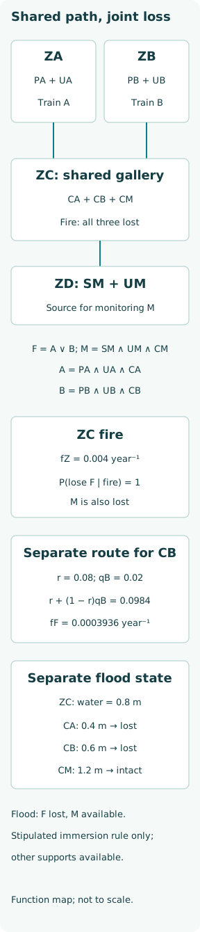
Consider a generic service system with two trains, A and B. Either train can provide cooling function F for the defined mission. A train needs its pump P, local supply U and command cable C. Monitoring function M needs sensor module SM, supply UM and communication cable CM. The example concerns availability of these functions, not a quantified consequence such as injury or asset loss.
Write the success logic as F = (PA ∧ UA ∧ CA) ∨ (PB ∧ UB ∧ CB), and M = SM ∧ UM ∧ CM. The symbols mean that an element remains capable of its required function in the hazard scenario. All unlisted controls and supports are fixed available here. Their omission is a boundary assumption, not evidence that they are unimportant or independent in a real system.
Build a zone-to-equipment-to-function register
Place pump PA and supply UA in zone ZA, and PB and UB in ZB. Both command cables and monitoring cable CM cross gallery ZC. The monitoring source SM and its supply UM are in ZD. The table records functional links as well as equipment locations; otherwise the two separated pump symbols can conceal the single gallery on which both train paths depend.
| Zone | Equipment | Function link |
|---|---|---|
| ZA | PA, UA | A train |
| ZB | PB, UB | B train |
| ZC | CA, CB, CM | A, B and monitoring paths |
| ZD | SM, UM | Monitoring source |
The NRC/EPRI fire-PRA method links equipment-associated cables to compartment locations. That mapping principle is used here without importing its nuclear assumptions. A route should identify every relevant segment and interface, not only the room containing the equipment’s nameplate. The same component may be vulnerable in several zones through its cables, utilities or physical attachments.
Define a damaging fire scenario in the gallery
Assign the invented damaging-gallery-fire scenario a frequency fZ = 0.004 year⁻¹. Conditional on this already-defined damaging scenario, CA, CB and CM are all lost with certainty. This is not the frequency of every small ignition in the gallery; detection, suppression and fire growth have been folded into the chosen scenario boundary. No additional generic suppression multiplier is applied later.
The fire need not destroy either pump mechanically. Setting both command paths to unavailable is sufficient to make both train terms false, so F is lost. CM loss also makes M unavailable. Thus the same explicit spatial event defeats cooling and monitoring together. Recording three independent cable failures would obscure both the initiating mechanism and the dependence between the functional losses.
Calculate the original hazard contribution
The conditional probability of losing F in this gallery-fire scenario is unity, and the resulting contribution is 0.004 year⁻¹. Monitoring is also lost conditional on the same event. These are concurrent consequences of one scenario, not separate independent initiating events to be multiplied. Counting the same gallery fire once for cooling and once for monitoring also does not create two distinct site events.
Suppose someone instead used a nominal train unavailability of 0.02 for each train and calculated 0.004 × 0.02² = 0.0000016 year⁻¹. That number answers an inappropriate independent-train question. It ignores the scenario-conditioned loss of both command paths. The error is in mapping the hazard to the logic, not merely in choosing an insufficiently conservative common-cause coefficient.
Compare a physically separated alternative
Now consider a hypothetical design alternative in which CB avoids ZC and runs within the protected B-side route. Leave every other mapping unchanged. A gallery fire still defeats CA and CM. Train B can now remain available if the hazard does not propagate to ZB and its remaining required elements perform. This is a model comparison, not an instruction to reroute a real installation.
Assign r = 0.08 to damaging propagation into ZB given the gallery fire. Conditional on no propagation, assign qB = 0.02 to failure of the remaining B train during the mission. The conditional structure matters: qB is not another independent fire-spread probability. It applies only on the no-spread branch and includes the stipulated residual availability of that complete remaining train.
Calculate the remaining dependence explicitly
The alternative conditional loss is P(loss F | ZC fire) = r + (1 − r)qB = 0.0984. Its annual contribution is 0.0003936 year⁻¹. The propagation branch contributes 0.00032 year⁻¹; no propagation followed by residual B failure contributes 0.0000736 year⁻¹. Their sum gives the total without counting a failed B train again on the branch where propagation has already defeated it.
Physical separation has changed this example substantially, but it has not removed all dependence. Monitoring M is still lost because CM remains in ZC. A manual recovery claim that requires that monitoring cannot simply be added unchanged. The assumed value of r needs hazard-specific evidence concerning the real propagation path and barrier state before the alternative can support an engineering decision.
Apply a different exposure map for flooding
Use the original route arrangement again for a separate, static flood illustration. Put vulnerable connectors CA, CB and CM at critical elevations 0.4, 0.6 and 1.2 m above the same local datum. Stipulate a water level of 0.8 m in ZC and a simple immersion rule: connectors at or below the level fail; higher connectors remain available. No flood-event frequency is assigned.
Under those assumptions, CA and CB fail while CM survives. Cooling F is lost, but monitoring M remains available. The fire and flood target sets therefore differ even though the zone name is identical. This elevation-only model excludes spray, humidity, dynamic loads, drain behaviour and propagation. It is a diagnostic illustration of mapping, not a claim that an elevated connector is flood-qualified.
Model boundaries and propagation as evidence claims
IAEA’s revised guide addresses fire propagation and, for flooding, equipment elevations, barriers and routes between areas. The useful question is whether the selected physical event can reach each required component during the mission. A line on a room drawing does not establish separation when an opening, cable penetration, shared drain or ventilation path can transmit damaging conditions.
Retain the state of doors, penetrations and relevant barriers in the scenario assumptions. Identify whether the hazard directly disables a component, causes spurious operation, or removes access needed for recovery. These mechanisms can have different timing and functional effects. A simple target-set model is appropriate only when its conservative or approximate treatment is understood and the important excluded mechanisms remain visible.
Separate explicit spatial loss from residual common cause
A gallery fire modeled as a common physical event should not also be counted inside an undifferentiated residual common-cause term for the same failures. Review the data boundary and event classification before combining the two. Residual common cause can still represent other shared mechanisms, such as a maintenance defect, provided those events and the explicit hazard scenario are distinguished consistently.
Likewise, unrelated background failures may remain possible on a hazard branch, as qB represents in the alternative. This does not restore independence to the hazard-induced losses. Use the conditional state of the surviving equipment and shared services. If dependencies cannot be resolved with a compact map, retain them in a joint model instead of assuming that different equipment identifiers imply independent availability.
Verify the physical map against the logic
An auditable review traces each function to its required equipment, each item to all vulnerable locations, and each scenario to a time-bounded target set. Compare that register with current drawings and a focused walkdown. Changes in cable routing, temporary openings, supply arrangements or equipment elevations can invalidate a previously correct map even when the fault-tree diagram has not changed.
Keep the original and alternative results beside their assumptions: loss of cooling, loss of monitoring, propagation state and residual failures. Neither total is a plantwide risk estimate or a barrier specification. The transferable insight is that redundancy belongs to complete functional paths exposed to a physical event, not merely to the count of pumps or rooms on a simplified schematic.