Knowledge / Risk analysis methods
Structured expert elicitation for PSA: evidence, ranges and disagreement
Frame the question, preserve individual uncertainty judgments and aggregate complete distributions transparently without disguising opinions as failure observations.
On this page
When a risk model needs a parameter that available evidence cannot estimate adequately, asking an experienced person for “the best number” leaves much of the reasoning invisible. Structured elicitation records the question, evidence, uncertainty and disagreement. This original three-expert exercise follows those records into an explicit probability pool and shows why averaging upper quantiles gives a different answer.
Define what the experts are judging
Let q be the unknown long-run probability that a temporary support function fails its defined 30 min mission after a particular utility-loss demand. Fix the equipment configuration, staffing, access state, environment and success criterion before asking for a judgment. The mission duration is an invented analysis boundary, not a response requirement for real equipment. A different demand or access state would be a different question.
NRC’s expert-elicitation publication describes judgments as a complement to data, analysis and experimentation. Here all experts, evidence-packet details and numerical judgments are fictional. The exercise develops an uncertainty input; it does not manufacture a measured failure rate. Evidence that could support direct estimation should still be collected and assessed for applicability.
Prepare a shared evidence packet
For this example, define a hypothetical packet with three labelled items: P1 is a configuration drawing that identifies the support interfaces; P2 is an equipment capability description that does not establish end-to-end deployment performance; P3 is an explicit gap register for degraded visibility, access restrictions and unfamiliar connections. These are constructed case assumptions, not reports from an actual installation.
Each expert receives the same version and records which items support or weaken each inference. Distinguish what a document states from what the expert extrapolates. A component capability claim cannot establish the whole mission if mobilisation, connection and support availability are absent from its scope. If an important condition is undefined, refine the question before trying to absorb the ambiguity into a wider number.
Select perspectives and prepare probability judgments
Use fictional expert A for equipment behaviour, B for task integration and C for site logistics. The labels describe complementary perspectives, not ranks or voting power. Record relevant experience, conflicts and missing expertise in a real exercise. Familiarity with one component does not guarantee competence about every part of the mission, and agreement among similarly trained experts may reflect a shared blind spot.
EFSA’s elicitation guidance structures the work around framing, expert selection, uncertainty elicitation, aggregation and documentation. For this exercise, first explain the difference between uncertainty about q and variability in future success or failure. Ask experts to consider evidence that would make q lower or higher before settling on a central estimate, and retain their reasons rather than only a fitted curve.
Record individual distributions and ranges
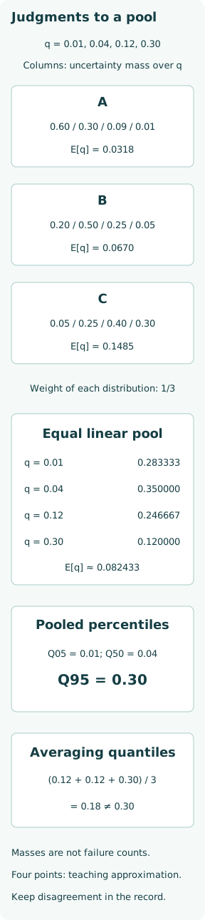
Use a deliberately coarse common support q = 0.01, 0.04, 0.12 and 0.30. Each expert assigns uncertainty mass across those four values. This finite approximation makes the arithmetic transparent; it is not a recommendation to put zero probability on all other possible values in a real assessment. Tail coverage and the choice of grid would themselves require review.
| Expert | q=0.01 | q=0.04 | q=0.12 | q=0.30 | E[q] |
|---|---|---|---|---|---|
| A | 0.60 | 0.30 | 0.09 | 0.01 | 0.0318 |
| B | 0.20 | 0.50 | 0.25 | 0.05 | 0.0670 |
| C | 0.05 | 0.25 | 0.40 | 0.30 | 0.1485 |
Each row sums to unity. The values in the four middle columns are judgments about the uncertain parameter, not observed demand counts. A emphasises the bounded equipment task; B gives more weight to interface uncertainty; C emphasises unresolved logistics. Under the stated discrete convention, their central 90% intervals are [0.01,0.12], [0.01,0.12] and [0.01,0.30], respectively. Discreteness can make actual enclosed mass exceed 90%.
Declare the aggregation rule before using it
Apply an equal-weight linear pool: at each support value, take the arithmetic mean of the three masses. The pooled masses are 0.283333, 0.350000, 0.246667 and 0.120000, shown rounded to six decimals. This is a mixture of distributions. It does not multiply expert beliefs as though the three people supplied independent failure experiments, and it does not assert that the experts agree.
The individual means are 0.0318, 0.0670 and 0.1485; the pooled mean is approximately 0.082433. Equal weighting is a transparent choice for this example, not a universal optimum. A performance-weighted scheme would require a separately justified calibration design and relevant evidence. Seniority, confidence of delivery and desired project outcome are not numerical calibration results.
Derive pooled quantiles from the pooled distribution
Define a quantile as the smallest support value at which cumulative mass reaches the requested probability. The pooled cumulative masses are 0.283333, 0.633333, 0.880000 and 1.000000. Therefore its 5th percentile is 0.01, its median is 0.04 and its 95th percentile is 0.30. These values express uncertainty about q under the chosen pool.
The individual 95th percentiles are 0.12, 0.12 and 0.30. Their average is 0.18, which is not the pooled 95th percentile. Quantiles are generally nonlinear functions of a distribution. Averaging three reported upper limits and calling the answer a pooled uncertainty limit would discard the actual mixture. Retain complete individual distributions or enough justified structure to reconstruct them.
Preserve disagreement after discussion
EFSA’s uncertainty methods distinguish mathematical pooling from group-based aggregation and keep unresolved disagreement visible. In this exercise, discussion could reveal that C imagined restricted access while A assumed unrestricted access. That would be a framing mismatch to resolve, not legitimate uncertainty to average away. If all judged the same conditions but interpreted incomplete evidence differently, the disagreement remains relevant.
Save initial judgments, any revisions and the reasons for revision. An expert may change a distribution after learning a previously overlooked fact, yet need not move toward the group mean. A useful record can show consensus on the question alongside disagreement on the answer. The pooled curve is a declared analytical representation, not a replacement for that record or proof that uncertainty has disappeared.
Propagate the uncertainty into a bounded PSA branch
For illustration, fix the compatible initiating-event frequency at 0.08 per operating year and let every modeled mission failure meet the named endpoint. Conditional on q, the endpoint frequency is 0.08q. Its pooled mean is approximately 0.006595 per operating year, while its 5th and 95th percentiles are 0.0008 and 0.024. Positive scaling preserves the discrete quantile ordering.
These are epistemic uncertainty summaries of a frequency, not a forecast interval for the number of failures next year. Event-count variability would need a separate model. Nor do they cover uncertain initiation frequency, other operating states or model omissions. If several branches share this same uncertain q, sample or propagate it consistently; independently resampling a common parameter changes the model.
Test aggregation sensitivity and evidence value
As a sensitivity only, assign A and B weights 0.25 each and C weight 0.50. The pooled mean becomes 0.09895. That difference shows the effect of the weighting choice; it does not establish that the revised pool is better calibrated. Keep both the rule and the numerical effect visible rather than choosing weights to obtain a preferred risk result.
The disagreement suggests a targeted evidence question: which part of the end-to-end support mission creates uncertainty about the upper tail? A configuration review, representative task demonstration or properly scoped operational dataset could address different gaps. Decide what evidence would discriminate among the competing reasons. Repeating the same opinions in another meeting is not equivalent to obtaining new information.
Leave a reproducible elicitation record
The record should retain the exact question, evidence versions, expert-selection rationale, training, individual judgments, rationale, changes, pooling rule and sensitivity results. Check that masses sum to unity, probabilities stay within their valid range and the pooled quantiles are recalculated from the full distribution. Preserve unresolved conditions as separate questions when they cannot credibly share one parameter.
This exercise ends with a transparent input and visible disagreement, not a claim of measured reliability. It precedes any later Bayesian update from new observations and differs from drawing a dependency network. The useful output is the traceable route from evidence and judgment to the exact uncertain quantity the PSA branch actually needs.