Accelerated life tests: stress models, mechanism changes and extrapolation

Choose the mechanism before choosing the hottest test

Consider a fictional polymer-sealed sensor whose specified failure endpoint is loss of insulation performance after a thermally activated degradation process. The example assumes that this process controls the endpoint in service and in every accepted test cell. A cracked seal, a melted adhesive and electronic overstress cannot be pooled merely because they all make the same sensor fail a functional check.

The experimental objective is to learn a life distribution at the stated use condition, not simply to create the largest possible number of failures. Failure analysis must accompany the life records: location, damage appearance and a credible physical pathway help distinguish acceleration of the intended mechanism from creation of another one. No numerical acceleration factor repairs an incorrect mechanism assignment.

Define what the acceleration factor actually scales

Let ηu be a life-scale parameter at use temperature Tu and ηs the corresponding parameter at stress temperature Ts. Define AF = ηu/ηs. Under a common time-scale acceleration model, the use lifetime distribution is the stress distribution stretched along the time axis by AF. An AF above unity means that the higher-temperature cell reaches corresponding quantiles sooner.

The Arrhenius model relates the factor to reciprocal absolute temperatures: AF = exp[(Ea/k)(1/Tu − 1/Ts)]. Ea is activation energy in eV and k is the Boltzmann constant in eV/K. This is a model for the selected mechanism and stress range. It is not a universal rule that every kind of failure accelerates by the same factor.

Keep the temperature and energy units consistent

Use 40 °C = 313.15 K and 85 °C = 358.15 K. For this calculation take k = 8.617333262 × 10⁻⁵ eV/K, a rounded physical constant. Dividing Ea by k gives kelvin; multiplying by a reciprocal-kelvin difference makes the exponential argument dimensionless. Substituting Celsius values in the reciprocal terms changes the model and is physically wrong.

Temperature means the temperature where the degradation occurs. A chamber setpoint is not automatically the specimen’s seal, junction or internal hot-spot temperature. Record stabilization, gradients and measurement uncertainty. If self-heating changes with stress or duty, a nominally single-temperature experiment may actually vary another stress at the same time. That confounding can be mistaken for an activation-energy effect.

Calculate one original central scenario

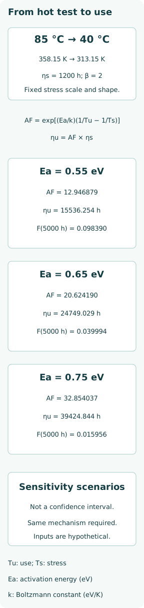
Assume Ea = 0.65 eV and a fictional stress-cell Weibull scale ηs = 1200 h at 85 °C. The temperature pair gives AF = 20.624190, so ηu = 24749.029 h at 40 °C. These are assumed model inputs and computed outputs, not an observed sensor lifetime or a supplier qualification. Rounding occurs only when presenting the result.

For a Weibull distribution, scale and shape jointly determine reliability. With a common shape β = 2, F(t) = 1 − exp[−(t/η)²]. The use-condition failure probability by 5000 h is 0.039994. The scale is the characteristic life, not the mean or a guaranteed minimum life. Reporting only the scaled hours would hide the distribution needed to interpret a mission claim.

Expose activation-energy sensitivity before celebrating the factor

Keep ηs fixed and substitute Ea = 0.55 eV and 0.75 eV. The acceleration factors become 12.946879 and 32.854037. Corresponding use scales are 15536.254 h and 39424.844 h, with 5000 h failure probabilities 0.098390 and 0.015956. A modest change in the assumed energy substantially changes the extrapolated answer.

These endpoints are a one-parameter sensitivity range, not a confidence interval. The direction also matters: when the high-temperature scale is held fixed, larger activation energy predicts a larger separation between hot and cool life. Real fitted scale and activation energy can be correlated, so their joint uncertainty cannot be reconstructed by combining individually convenient extremes without a statistical model.

Design stress cells that can test the bridge

At the central energy, hypothetical cells at 65 °C, 85 °C and 105 °C have factors 5.934688, 20.624190 and 62.824955 relative to 40 °C. This calculation shows their different information and duration demands; it does not authorize those temperatures for the material. The highest cell is useful only if it preserves the same relevant degradation mechanism and failure definition.

NIST’s test-planning guidance calls for multiple stress cells and avoiding stresses that introduce new mechanisms. A lower-stress cell closer to use can help check an otherwise long extrapolation, but it may need more units or more time to produce useful failures. Random allocation and consistent specimen preparation help separate stress effects from batch, chamber or manufacturing differences.

Preserve censoring and fit the cells together

Each specimen record needs its actual stress history, failure or censoring time, endpoint and mechanism diagnosis. A survivor at scheduled test closure contributes information that life exceeded its observed time. Dropping survivors or pretending every test ended in failure biases the fitted scales. A specimen withdrawn because it was visibly deteriorating is not automatically equivalent to administrative test closure.

A joint likelihood can estimate acceleration and life-distribution parameters while retaining censored observations. Compare the common-shape restriction with cell-specific alternatives and inspect residual structure and failure analyses. Failure to reject a restriction with a small sample is weak evidence of adequacy. A highly precise fit within hot cells can still leave the service extrapolation poorly constrained.

Treat a mechanism change as a model boundary

Suppose the hottest cell shows adhesive flow that is absent from the cooler cells and implausible at the use temperature. Its short lives may describe a new process. Combining them with insulation degradation can distort both the fitted slope and the apparent acceleration. Investigate the mechanism, define a justified admissible stress range and explain any revised analysis population before reporting a use prediction.

Excluding an inconvenient cell solely because it spoils a straight line is not a physical argument. Conversely, forcing a known different mechanism into one line is not conservative by default. Separate mechanisms may require competing-risk treatment and different stress relations. Preserve the excluded observations and reasons so the claimed service mechanism can be challenged without losing the underlying evidence.

Translate uncertainty into the actual service question

The illustrative 5000 h prediction assumes constant 40 °C mechanism temperature, fixed duty and no competing cause. A voyage temperature cycle, humidity change or vibration exposure is a different input. A variable-temperature calculation may need a validated damage-accumulation model; using the average Celsius temperature inside an exponential relation generally does not represent the full history.

Propagate uncertainty in life scale, activation energy, shape and temperature, including their dependence, and assess plausible alternative models. A confidence interval conditional on Arrhenius and a common shape does not cover arbitrary mechanism changes. Distinguish statistical estimation uncertainty from uncertainty about the physical extrapolation itself. The useful output is a mission probability or life quantile with those conditions attached.

Set a stopping boundary for the extrapolation claim

A defensible report identifies the tested material and configuration, specimen temperatures, accepted cells, failure mechanism evidence, censoring rules, fitted model and distance to service conditions. It states which features were tested and which were assumed. The original calculation here is reproducible, but its inputs deliberately contain no evidence that a real sensor has the selected energy or common shape.

Use the sensitivity result to decide which uncertainty would be worth reducing: a nearer-use cell, better specimen-temperature measurement or stronger failure analysis may be more valuable than extending an extreme-stress run. The engineering claim should stop where the mechanism or stress model ceases to be supported. Fast failures are useful only when their relation to the intended service failure remains credible.

Sources

1. NIST/SEMATECH — Arrhenius acceleration model.
2. NIST/SEMATECH — Accelerated life tests.
3. NIST/SEMATECH — Maximum likelihood for acceleration models.
4. NIST/SEMATECH — Weibull reliability model.