Operating-condition covariates in reliability: proportional hazards and causal limits

Define the failure endpoint and comparison population

Follow new units from entry into operation until the first specified functional failure. Age t is measured in operating hours; no repair is credited within the mission. Let z = 0 identify the reference duty group and z = 1 a higher-duty group assigned at the start and held fixed in the initial example. The labels describe hypothetical groups, not observed test results.

The groups must share a usable endpoint and exposure definition. If a warning in one group triggers removal while the other remains in service until breakdown, their recorded failure times are not directly comparable. Starting observation on already aged units also requires the prior survival and entry age to be handled correctly. Define the risk set before interpreting a coefficient as a difference in reliability.

State what proportional hazards actually assumes

Use h(t | z) = h0(t) exp(βz), where h0(t) is the baseline hazard in inverse hours and β is dimensionless for the binary duty indicator. NIST describes proportional hazards as a covariate-dependent multiplier of a baseline hazard. For two fixed groups differing only in z, their hazard ratio is exp(β) at every age where the ratio is defined.

This assumption permits the baseline hazard itself to rise, fall or change shape over time. It constrains the ratio between the compared hazards, not each hazard to be constant. A fitted Cox model can leave baseline shape unspecified when estimating relative effects, but absolute mission survival still needs an estimated baseline cumulative hazard. A hazard ratio by itself cannot give the probability that a unit completes its mission.

Build a fully specified original duty example

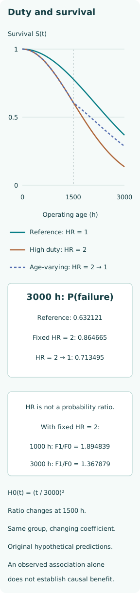
Assume β = ln(2), so the higher-duty group has hazard ratio 2. Choose baseline cumulative hazard H0(t) = (t/3000)², with time in hours. This is a Weibull baseline with shape 2 and scale 3000 h, consistent with the standard Weibull cumulative-hazard and survival forms. These parameters are invented for explanation and are not estimates of a real operating load effect.

At 1000 h, baseline cumulative hazard is 0.111111 and the higher-duty value is twice as large. At 3000 h, the corresponding baseline value is 1. Multiplying hazard by the duty factor multiplies the cumulative hazard for a covariate held fixed through the interval. That rule does not automatically extend to a condition that changes during the mission; its exposure history must then enter the integration.

Convert the multiplier into absolute mission probabilities

For a fixed covariate, S(t | z) = exp[−H0(t) exp(βz)] = S0(t) raised to exp(βz). At 1000 h, reference survival is 0.894839 and higher-duty survival is 0.800737. The respective failure probabilities are 0.105161 and 0.199263. All displayed probabilities are rounded to six decimals; the hazard ratio remains 2 in the assumed model.

At 3000 h, reference survival is 0.367879 and higher-duty survival is 0.135335. Their failure probabilities are 0.632121 and 0.864665. The cumulative failure-probability ratios are 1.894839 at the shorter horizon and 1.367879 at the longer one. Neither equals the hazard ratio. Doubling a rate among survivors does not double the fraction of the original population that has failed by every horizon.

Give continuous covariates meaningful reference units

To add temperature, define x = (T − 40)/10 with T in degrees Celsius, then write h(t | z,x) = h0(t) exp(βz + θx). Set the fictional coefficient θ = ln(1.5). The associated multiplier is 1.5 per 10 °C increase, conditional on duty and the other modeled variables. Centering at 40 °C makes h0 the reference-duty hazard at that stated temperature.

For high duty at a fixed 50 °C, the joint multiplier is 2 × 1.5 = 3 if the additive log-hazard form and absence of interaction are appropriate. At 1000 h this gives failure probability 0.283469. The unit definition matters: reporting θ without saying whether temperature is in single degrees or 10 °C increments changes the interpretation. Extrapolating this log-linear relationship beyond observed temperatures also needs justification.

Test an effect that changes with age

As a separate original counterexample, keep z fixed but let the high-duty hazard ratio equal 2 through 1500 h and 1 afterward. This changes the coefficient with age; it does not mean the unit changed duty at that instant. At 3000 h its cumulative hazard is 2H0(1500) + [H0(3000) − H0(1500)] = 1.25, giving failure probability 0.713495 and survival 0.286505.

The constant-ratio model instead gives failure probability 0.864665 at that horizon. A single fixed coefficient cannot reproduce the counterexample’s early and late hazard ratios simultaneously. When the later ratio becomes unity, the survival curves do not instantly become equal: the earlier cumulative exposure remains. An age-specific rate comparison and a full-mission probability therefore answer different questions even in a completely specified mathematical model.

Check proportionality with evidence across the relevant ages

The survival package’s proportionality diagnostics use scaled Schoenfeld residuals and a time-dependent coefficient plot. Under the assumed fixed effect, the underlying coefficient function should be horizontal. Examine age patterns and uncertainty alongside a formal test, rather than treating a large p-value as proof that the effect is constant. Sparse late failures can leave substantial departures difficult to detect.

No fit, residual plot or hypothesis test has been performed on observed data in this example. For an actual fleet, assess each relevant covariate, the baseline shape used for prediction and whether the available exposure spans the intended mission. A time interaction, age bands or stratification can be appropriate responses to nonproportionality, depending on the question. Their parameters and resulting absolute predictions still need validation.

Distinguish changing conditions from changing coefficients

A time-varying covariate z(t) records an actual change in operating conditions, while β(t) represents a change in the association for the same covariate contrast as units age. With changing conditions, integrate h0(u) exp[βz(u)] over the actual history. Replacing that history with a lifetime average can lose the ordering of exposure, especially when the baseline hazard increases with age.

Use only covariate information available at each risk-set time. A sensor average computed using values after failure or a label based on eventual maintenance cannot be treated as known at installation. If operators reduce load in response to deterioration, the exposure is also connected to impending failure. A convenient time-updated regression does not by itself resolve that feedback or identify what would happen under an imposed duty policy.

Keep association, intervention and survivor selection separate

Higher-duty units may differ in production batch, site temperature, maintenance resources or the reasons they were assigned demanding work. Adjusting for recorded covariates can improve a conditional prediction but does not guarantee that changing duty alone would change failure by the fitted multiplier. A causal claim needs a defined intervention, appropriate comparison design and defensible assumptions about confounding, exposure measurement and follow-up.

Hazard-ratio interpretation also conditions on the units still surviving at each age. The surviving groups can differ from their starting populations as susceptible units fail earlier. Thus even a carefully estimated rate contrast is not automatically an individual causal effect or a marginal mission-risk ratio. If the engineering decision is a duty change, state the desired counterfactual mission outcome and evaluate evidence for that question explicitly.

Make a prediction useful within its supported scope

Report the endpoint, age clock, reference group, covariate units, baseline cumulative hazard, coefficients and supported operating range together. Include uncertainty in both relative effects and the baseline when predicting absolute reliability. Administrative censoring may be acceptable under suitable conditional independence assumptions; removal driven by incipient failure may not be. Recurrent repairs and competing endpoints need models consistent with their distinct targets.

The original example checks the identity between hazard integration and survival, the unequal hazard and cumulative-risk ratios, and a concrete failure of proportionality. A real application adds calibration on relevant units, sensible handling of missing exposure and checks after operating conditions change. Use the model to describe what the evidence supports, then keep any claim about the benefit of intervention tied to evidence capable of answering it.

Sources

1. NIST/SEMATECH — Proportional hazards model.
2. NIST/SEMATECH — Weibull reliability model.
3. R survival documentation — Test the proportional hazards assumption of a Cox regression.
4. Miguel A. Hernán — The Hazards of Hazard Ratios.
5. Therneau, Crowson and Atkinson — Using Time Dependent Covariates and Time Dependent Coefficients in the Cox Model.