Imperfect-repair models: virtual age and the degree of restoration

Separate operating age, calendar age and virtual age

An asset can accumulate operating hours, spend calendar time awaiting parts and carry damage from earlier service. These clocks need not advance together. Here x is time spent operating between successive failures, measured in hours. Repair downtime is excluded from the numerical clock. Virtual age v is a model state, also in hours, representing the age at which the baseline failure mechanism behaves after a repair.

Virtual age is not a directly observed reading on the hour meter. An overhaul does not reverse elapsed calendar time, and a reset controller does not prove that cracks or wear were removed. If corrosion continues while stopped, excluding downtime needs a separate physical justification or an additional aging state. Define the clock before interpreting a fitted restoration factor or comparing maintenance strategies.

Write the repair rule before naming its factor

Use the type II rule vi = q(vi−1 + xi), beginning with v0 = 0. Between repairs, virtual age increases one hour per operating hour. The dimensionless q is the retained fraction of pre-repair virtual age: q = 0 gives perfect restoration and q = 1 gives minimal repair. Values between these endpoints retain part of the accumulated age. A smaller q therefore means stronger rejuvenation in this convention.

Virtual-age models distinguish the age just before and just after each repair and evaluate intensity at that state. Some publications parameterize the fraction removed instead, reversing the meaning of a larger coefficient. Report the equation with the parameter, not just “repair effectiveness.” In this model q is neither the probability that a technician succeeds nor the fraction of replacement parts installed.

Trace a conditional three-repair history

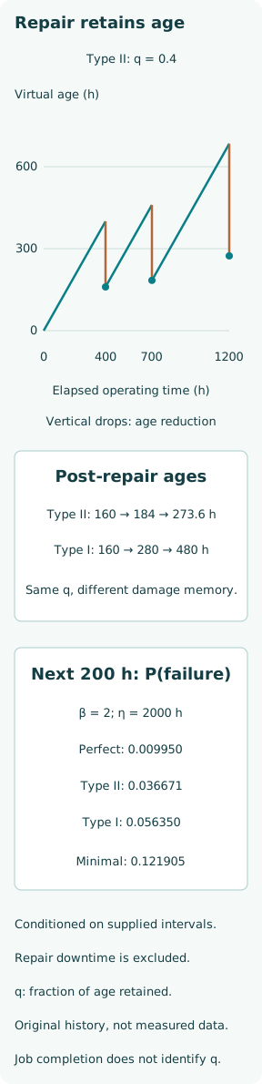
Consider fictional inter-failure operating intervals of 400 h, 300 h and 500 h. With q = 0.4, the first repair changes virtual age from 400 h to 160 h. The next interval raises it to 460 h and the second repair reduces it to 184 h. The final interval raises it to 684 h, followed by a third repaired state of 273.6 h.

Total elapsed operating time is 1200 h, whereas the post-repair virtual age is much smaller. This is a conditional bookkeeping example using a supplied history, not a simulation asserting that different repair policies would produce those same failure times. A full policy comparison must generate or integrate each policy’s failure history under its own intensity and include repair costs, downtime and any replacement decisions.

Compare perfect, minimal and weaker restoration

Applying q = 0 at every repair gives post-repair ages 0 h, 0 h and 0 h. With q = 1, the ages are 400 h, 700 h and 1200 h. These endpoints reset all accumulated model age or preserve it entirely. Minimal repair restores the failed function while leaving the modeled aging condition at its pre-failure level; it does not mean no physical work occurred.

For q = 0.7, the corresponding ages are 280 h, 406 h and 634.2 h. These are larger than the q = 0.4 ages because more age is retained at every intervention. The comparison assumes that the same baseline mechanism remains valid after all repairs. A modification that changes the mechanism, material or operating environment may require new baseline parameters as well as an age update.

Turn the state into a next-failure probability

Choose an original Weibull baseline with shape β = 2 and scale η = 2000 h. Its cumulative hazard is H0(a) = (a/η)² and its hazard is h0(a) = 2a/η². NIST gives the Weibull hazard and cumulative-hazard forms. After a repair ending at age v, no further failure over u hours has conditional probability exp[−{H0(v + u) − H0(v)}].

For v = 273.6 h and u = 200 h, the integrated hazard increment is 0.03736 and the next-interval failure probability is 0.036671. The immediate post-repair hazard is 0.0001368/h. That rate is not the 200 h probability, and multiplying it by the interval would ignore the increasing hazard during operation. The calculation concerns the first subsequent failure, with no intervention before it.

Check how restoration changes the same forecast horizon

Over the next 200 h, perfect restoration gives failure probability 0.009950 and minimal repair gives 0.121905. The q = 0.7 state gives 0.070790, between the q = 0.4 and minimal cases. These are conditional probabilities at the third repair under the specified increasing-hazard baseline. They are not annual failure frequencies, cumulative counts or availability estimates for a continuously repaired fleet.

A zero immediate hazard at v = 0 in this Weibull model does not imply a failure-free future interval: hazard rises as operating time resumes. Conversely, a nonzero retained age need not imply worse short-term reliability under every baseline shape. The ordering here relies on increasing hazard. If the physical failure mechanism has early-life hazards or multiple aging regimes, scrutinize the meaning of rejuvenation before transferring that ordering.

Distinguish reduction of all age from reduction of the latest interval

The type I alternative is vi = vi−1 + qxi. At q = 0.4, the same supplied intervals give post-repair ages 160 h, 280 h and 480 h. Only the age accumulated since the preceding repair is partially removed; earlier retained age remains. The next 200 h failure probability after the third repair is then 0.056350, larger than the type II result.

Both rules agree at the first repair and at their constant perfect and minimal endpoints from a new start. They diverge after repeated partial repairs because they encode different memory of earlier damage. The same numeric q is therefore not interchangeable between models. Replacing a recently worn seal while leaving the older housing unchanged may call for a different age structure from refurbishing the complete assembly.

Recognize what a completion record cannot identify

A completed repair record establishes an intervention time and perhaps its scope. It does not identify q. Estimation needs ordered failures, operating exposure, censoring and useful information about repair type and duty. Baseline aging and rejuvenation can partly compensate for each other in a short sequence: a steeper baseline with stronger restoration may resemble a flatter baseline with weaker restoration over the observed range.

There is a sharp limiting example. If the baseline is exponential with constant hazard, H0(v + u) − H0(v) does not depend on v. Failure times in this age-only model then contain no information about q, even with exact repair timestamps. An age reset may still matter physically through mechanisms absent from that baseline, but the chosen statistical model cannot infer it from an invariant intensity.

Preserve recurrence history when checking the model

Do not pool all intervals as independent new-unit lifetimes unless perfect renewal is justified. NIST’s power-law repairable-system model describes a recurrence rate; a similar algebraic shape does not turn recurrence times into independent Weibull lifetimes. For partial repair, the preceding state enters the conditional distribution of each next interval. Asset identity and the order of interventions are part of the evidence.

Check predictions on later intervals and comparable assets, accounting for parameter uncertainty and the maintenance policy that generated the data. Early preventive removal, missing small failures or changes in duty can distort the apparent repair benefit. A good historical fit alone does not establish that the selected age rule remains valid after a new overhaul procedure. Predictions must be assessed where the proposed decision will use them.

Use restoration as a testable engineering hypothesis

Choose a restoration rule that matches the intervention’s physical reach, then evaluate alternative retained-age factors and baseline laws. Report what was replaced, what damage can remain and whether operating conditions changed. The simple scalar state is most credible when one aging mechanism dominates; mixed components may need separate ages, degradation measurements or a richer state model instead of one universal factor.

Keep the deliverable explicit: the supplied history, model equation, parameter convention, operating-hour basis and conditional forecast horizon. Check both endpoint rules and the cumulative-hazard difference numerically. A model that passes those checks can support a maintenance comparison, while evidence about restoration still comes from interventions and subsequent behavior. Closing a work order and demonstrating rejuvenation remain separate engineering achievements.

Sources

1. El-Aroui and Gaudoin — Imperfect repair models: sequential goodness-of-fit testing based on predictive performances.
2. NIST/SEMATECH — Weibull reliability model.
3. NIST/SEMATECH — Non-homogeneous Poisson process, power law.
4. ReliaSoft — Recurrent Event Data Analysis.