Load–strength reliability: mean safety margin and distribution overlap

Put load and strength on the same physical basis

Let S be the resistance expressed as an equivalent failure stress and L the stress induced by one specified load application, both in MPa. Define failure as L > S and the margin as M = S − L. This comparison is meaningful only when the stresses refer to the same location, temperature, loading mode and failure criterion. Force in newtons cannot be compared directly with a material stress in MPa.

A brittle fracture threshold, a yield limit and a fatigue-life criterion are different endpoints. This example concerns an instantaneous threshold under one application, with no damage accumulation or change in resistance during that application. Geometry and concentration factors can be included in the transformation from force to L, but uncertainty in those factors then belongs in the joint model rather than disappearing inside a nominal stress.

Define exceedance rather than a shaded overlap area

The desired probability is pf = P(L > S). For independent continuous variables, it can be written as ∫ fS(s)[1 − FL(s)] ds: average the chance of exceeding a particular strength over all strengths. ReliaSoft’s stress–strength treatment defines failure through stress exceeding strength. Under dependence, replace the marginal load distribution with the appropriate conditional distribution given S.

The area where two marginal density curves visually overlap is not generally pf. That area measures similarity of distributions; exceedance concerns paired draws and their ordering. Two plots with identical load and strength marginals can therefore represent different failure probabilities if their dependence differs. A useful teaching figure plots the margin distribution and shades M below zero, because that shaded tail is the actual failure event.

Keep the average margin while changing the scatter

Use fictional means E(S) = 120 MPa and E(L) = 100 MPa for every case. The mean margin is 20 MPa and the ratio of means is 1.2. Neither number is a reliability or a guaranteed lower bound. In a narrow independent case, let the standard deviations be 6 MPa for strength and 8 MPa for load; in a wide independent case, double them to 12 MPa and 16 MPa.

Assume joint normality, not merely normal-looking individual histograms. A linear difference is then normal with mean 20 MPa. The normal CDF converts a standardized margin into a tail probability. Its support extends over all real values; using it for physical strengths and loads is an approximation whose plausibility must be checked, particularly if negative values or extreme tails are material to the decision.

Calculate the variance with its covariance term

For any finite-variance S and L, Var(M) = σS² + σL² − 2 Cov(S,L) = σS² + σL² − 2ρσSσL. This identity is exact for a linear difference; normality is needed for the normal-tail calculation, not for the variance identity. The covariance term has units MPa². Omitting it is an independence or zero-covariance assumption, not a neutral calculation setting.

NIST emphasizes paired measurements and the treatment of covariance. In practice, the association might reflect common temperature, matched manufacturing lots or how equipment is assigned to duties. Independent unpaired strength coupons and a separate duty histogram do not directly reveal the pairing. A selected value of ρ should therefore be a stated sensitivity assumption until the physical mechanism and relevant paired evidence support it.

Compare the original single-application probabilities

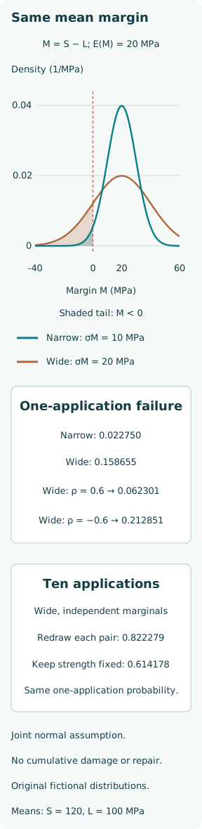
For joint normality, pf = Φ[−20/σM], where Φ is the standard normal CDF. The narrow independent margin has σM = 10 MPa and pf = 0.022750. The wide independent margin has σM = 20 MPa and pf = 0.158655. Values are rounded to six decimals. Equal mean safety margins and equal ratios of means thus coexist with substantially different threshold-exceedance probabilities.

Keep the wide marginal standard deviations and set ρ = 0.6. Then σM = 13.023056 MPa and pf = 0.062301. With ρ = −0.6, σM = 25.107768 MPa and pf = 0.212851. These are deliberately separate dependence scenarios, not estimates from a tested fleet. The figure retains the common mean while displaying how the margin tail moves across the failure threshold.

Interpret the sign without turning correlation into a design benefit

In this particular difference model with a positive mean margin, positive S–L correlation reduces margin variance: stronger units tend to see larger loads and weaker units tend to see smaller ones. Negative correlation does the reverse. This is a statement about the specified joint normal model. It is not a recommendation to increase operating load whenever a strength estimate is high, or proof that an observed correlation is causal.

Correlation alone does not describe arbitrary tail dependence. Outside joint normality, two joint distributions can share means, variances and correlation while giving different exceedance probabilities. A thermal mechanism might also shift the means or reshape tails, so varying only ρ would miss that effect. Retain the full joint distribution or a defensible conditional model when rare paired extremes govern the decision.

Give repeated applications their own sample space

For ten independently redrawn wide-case pairs, failure on at least one application is 1 − (1 − pf)¹⁰ = 0.822279. This model redraws both load and strength for every trial, as might describe separately sampled components. It does not describe ten applications to one unchanged component whose uncertain strength remains fixed. The single-application probability is the same, but the dependence between trials is different.

If S is drawn once and ten loads are independent of each other and of S, survival is E[FL(S)¹⁰]. Integrating the same wide normal distributions gives failure probability 0.614178. Weak units tend to fail repeatedly in the hypothetical trial sequence, while strong units tend to survive, producing dependent outcomes after averaging over S. Replacing the expectation of a power with a power of the expectation loses that structure.

Distinguish a maximum load from cumulative damage

The fixed-strength calculation is equivalently P(max Lk > S) over the specified ten applications. It assumes resistance does not decline, prior subthreshold applications cause no damage, and the load distribution remains unchanged. A life-cycle maximum needs a defined number of applications or an explicit stochastic arrival process. “Lifetime load” without a duration, count or duty description leaves the event undefined.

Fatigue, wear, corrosion and creep can reduce resistance or accumulate damage even when every individual load remains below an instantaneous threshold. Those mechanisms need a time-dependent resistance or damage model and an appropriate failure criterion. Merely increasing the count in an unchanged stress–strength equation does not create a fatigue model. Likewise, serially correlated loads require a joint maximum distribution rather than the independent-load power formula.

Separate scatter from uncertainty about the scatter

The displayed standard deviations describe assumed physical variability across the population or applications. Uncertainty in their estimates is another layer. A limited coupon program, sensor calibration error or missing high-duty operation can leave both tail shape and dependence poorly known. A probability calculated from fitted parameters is conditional on that fit; it does not automatically include parameter uncertainty or model-form uncertainty.

For a design review, vary the uncertain means, scales and dependence within physically justified alternatives and record which assumptions dominate. If the predicted failure probability is extremely small, central-data agreement offers little direct evidence about the relevant tail. Additional decimal places and a large simulation sample improve numerical precision while leaving that evidence gap unchanged. Quantify the uncertainty that matters before choosing a computationally elaborate estimator.

Connect the model to an engineering action

The example gives several distinct levers: raise resistance, lower the load distribution, reduce their scatter, or manage the matching between units and duties. A proposed action must be evaluated through the variables it actually changes. Screening weak units changes the retained strength distribution and may introduce measurement error; derating changes loads and possibly temperature-dependent strength. Reusing the original probability after either intervention is inconsistent.

Report the failure criterion, units, population, joint distribution, dependence assumptions and application horizon with the result. Check that failure grows as the load shifts upward or strength shifts downward under otherwise unchanged assumptions. Then decide whether the relevant intervention, evidence and acceptable probability all refer to the same event. A mean margin becomes useful when it sits inside that explicit reliability argument.

Sources

1. ReliaSoft — Life Data Analysis Reference, Stress-Strength Analysis.
2. NIST/SEMATECH — Normal distribution.
3. NIST/SEMATECH — Propagation of error considerations.