Reliability target allocation: from system budget to subsystem requirements

Allocate a mission target through an explicit series model, a reserved interface contribution and a constrained effort example, while keeping requirements separate from demonstrated performance.

On this page

A system target does not tell each subsystem team what to deliver. Allocation works backward from the required mission performance through a chosen architecture, then asks whether the resulting requirements are achievable and verifiable. An original three-subsystem example uses a logarithmic reliability budget to make that reasoning and its tradeoffs visible.

Define the requirement before dividing it

Suppose a fictional system must complete a 1000 h operating mission with reliability at least 0.96. Success requires subsystem A, subsystem B, subsystem C and an interface block all to remain functional. There is no credited repair during the mission. State the environmental profile, starting condition and failure criteria with this requirement; changing any of them changes what the target means.

Reliability is a probability of completing that mission, not uptime averaged over a repaired service life. The same numerical target at a different duration is a different requirement. A supplier’s calendar-year claim cannot be inserted without reconciling its exposure and endpoint. Allocation also needs a decision about which failure contributions belong to each subsystem, so connectors or shared control functions are neither omitted nor charged twice.

Use the architecture to choose the combination rule

The independent series model multiplies component reliabilities and fails at the first component failure. Here Rsys = RA RB RC Rint. Independence is a substantive assumption: shared power, a common thermal environment or failure propagation can invalidate it. Treating the interface as a separate block is meaningful only if its modeled contribution is defined consistently with the subsystem boundaries and dependence assumptions.

If the real system has standby units, switching, degraded operation or repair, this simple product may be inappropriate. Build the corresponding state or logic model before distributing the target. An importance ranking identifies sensitivity of a given model to component values; it does not uniquely prescribe requirements. Allocation additionally needs feasibility, resource and evidence constraints, which can favor a different distribution from a ranking alone.

Convert the product into an exact additive budget

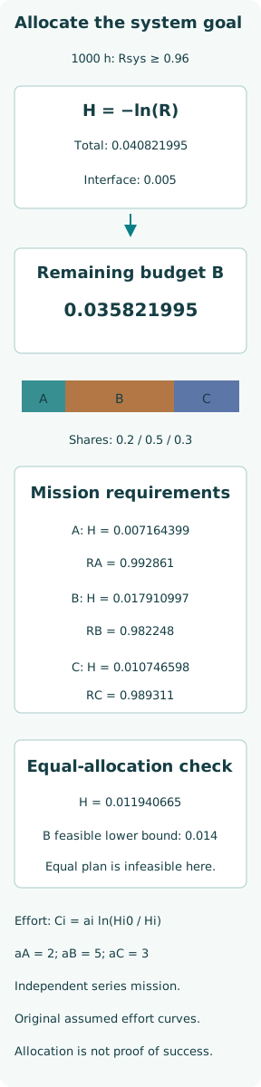
Define Hi = −ln(Ri), a dimensionless mission cumulative hazard or log-reliability debit. Then the target is HA + HB + HC + Hint ≤ −ln(0.96) = 0.040821995. This is an exact transformation of the independent series product. It does not require constant failure rates; each Ri can come from any compatible lifetime model at the stated mission time.

Reserve Hint = 0.005 for the explicitly modeled interface contribution. The remaining subsystem budget is B = 0.035821995. Reserve means this portion is unavailable to the other teams; it does not prove that unmodeled failures fit inside it. If all debit is assigned to hardware while integration failures are ignored, the apparent arithmetic closure hides an incomplete system boundary.

Specify what makes improvement difficult

Use original baseline debits HA0 = 0.020, HB0 = 0.035 and HC0 = 0.025. Together with the interface they imply baseline system reliability 0.918512, below the target. Assume the lowest attainable debits under the considered technologies are 0.006, 0.014 and 0.009. A lower debit means higher reliability, so these are lower bounds on H and upper limits on achievable reliability.

NASA describes allocation with explicit objectives and component feasibility constraints. For this example, introduce fictional effort Ci = ai ln(Hi0/Hi), with coefficients aA = 2, aB = 5 and aC = 3 effort units. The logarithm compares dimensionless quantities, effort is zero at baseline and rises as reliability improves. These are stipulated design-study curves, not measured supplier prices or an industry standard.

Derive a justified unequal allocation

Minimize total effort while meeting HA + HB + HC ≤ B and the stated bounds. Because more allowed debit reduces effort, the optimum uses the full available B. At an interior solution the marginal effort magnitudes ai/Hi are equal. Therefore Hi = B ai/(aA + aB + aC), giving shares 0.2, 0.5 and 0.3. The larger coefficient receives more allowed debit because reducing its debit is more expensive in this model.

The results are HA = 0.007164399, HB = 0.017910997 and HC = 0.010746598. Each lies between its feasible lower bound and its baseline, so no bound is active. Each effort curve has positive second derivative ai/Hi²; the feasible region is convex. Thus the interior stationary allocation is the global minimum for these assumed curves, rather than merely an unexplained weighted split.

Original allocation for a 1000-hour independent series mission. System target 0.96 gives log budget 0.040821995; interface uses 0.005 and leaves 0.035821995. Effort coefficients 2, 5 and 3 assign subsystem shares 0.2, 0.5 and 0.3, producing reliabilities 0.992861, 0.982248 and 0.989311. Equal allocation violates B’s feasible minimum debit. — Original constrained design example. All debits are dimensionless values of minus log reliability at the same mission; they are not failure probabilities. The weighted split follows from the stipulated convex log-effort objective and is feasible within the assumed bounds. Allocation does not demonstrate achieved reliability.

Translate each debit into a reviewable requirement

The corresponding mission reliabilities are RA = 0.992861, RB = 0.982248 and RC = 0.989311. Multiplying their unrounded values by exp(−0.005) gives 0.96. Total illustrative effort is 7.935742 units. Rounded display values are for communication; use full precision when checking the final product or writing a budget balance to avoid treating rounding drift as an engineering margin.

If each subsystem separately assumes constant hazard over 1000 h, its rate target would be Hi/1000, in inverse hours. That conversion is optional and conditional. It cannot establish a constant-hazard law from a mission reliability alone. A component with wear-out may satisfy this mission requirement while having a substantially higher instantaneous hazard near the mission end than its average log-debit rate suggests.

Test equal allocation against the actual constraints

An equal residual split would give every subsystem H = 0.011940665. It satisfies the sum algebraically, but asks B to beat its lowest feasible debit of 0.014. The equal plan is therefore infeasible under the stated technology limits. Its symmetry is not a justification. Conversely, equal allocation can be a sensible provisional choice when subsystems are comparable and evidence does not support a more detailed distinction.

Allocation methods distinguish equal, weighted and cost-based choices and make feasibility inputs explicit. The present unequal solution is optimal only for the invented log-effort functions and bounds. If qualification cost, mass, schedule or supplier constraints change, re-solve the problem. Assigning weights from expert judgment may be useful, but it should not be reported as a cost optimum without the matching objective and evidence.

Handle a budget overrun at system level

Suppose B later needs HB = 0.020 while A and C keep their allocated values and the interface reserve is unchanged. System reliability falls to 0.957997. The subsystem team cannot make the system meet its target by renaming that value a new allocation. A change requires an explicit trade elsewhere, a redesigned architecture or an authorized change to the system requirement.

One feasible numerical recovery is HA = 0.0065 and HC = 0.009321995, with HB = 0.020. All remain inside the original bounds and their sum returns to B. This demonstrates that a coordinated reallocation is possible; it does not assert that this particular recovery is the new effort optimum. The revised design and its verification burden must be evaluated before teams commit to the redistributed targets.

Keep numerical allocation separate from evidence of achievement

An assigned value is a requirement. A prediction from component data is a model result. A demonstration test gives evidence under a stated statistical plan. These objects can share a number without becoming interchangeable. Passing the product calculation proves consistency of the allocated values under the architecture; it does not prove that delivered hardware will attain them or that all environmental interactions are covered.

Write a verification approach beside each requirement, including mission definition, acceptance rule, uncertainty treatment and interface responsibilities. Separate subsystem tests at different duties do not automatically substantiate the system product. If reliability estimates have uncertainty, establish a coherent treatment of joint evidence and dependence rather than multiplying favorable point estimates and calling the result a demonstrated lower bound. System integration must remain part of the evidence plan.

Maintain the allocation as the design changes

A useful allocation record includes the system target, architecture, debit definitions, interface reserve, objective, feasibility limits and accountable subsystem owners. Revisit it when a supplier changes, the mission length grows, failure classification shifts or new common mechanisms are discovered. A target distributed early in design should evolve with evidence rather than surviving unchanged because a spreadsheet once balanced.

For the original example, the decisive checks are the exact log-budget closure, feasible component bounds and the assumptions behind the effort optimum. For a real project, the harder check is whether those assumptions describe what teams can build and verify. Treat allocation as an explicit agreement about design requirements and resources, then use independent performance evidence to determine whether the agreement has been achieved.