Knowledge / Risk analysis methods
Fault-tree top-event frequency: time in failure versus entries into failure
Calculate how often a repairable system enters its top event, distinguish occupancy from transition flow, and show how the same unavailability can hide very different interruption patterns.
On this page
A top-event probability answers a question about a defined state or mission. It does not automatically say how often the system enters that state. A repairable system can spend the same total fraction of time failed through a few long interruptions or many short ones. To count entries, the logic must be combined with the transitions that cross from outside the top event into it.
Name the quantity before manipulating the fault tree
Let Q(t) = P[T is true at time t]. This is dimensionless snapshot unavailability when T denotes the failed state. Let f_in(t) be the expected number of entries into T per unit time. It has units such as h⁻¹. A mission probability of ever reaching T is a third quantity and includes the path over an interval.
NASA’s handbook explains that the meaning of a top-event result depends on its definition and input basis. A report should therefore label the result explicitly. Multiplying a snapshot probability by the number of hours in a year gives expected failed hours under stationarity, not the number of failures.
Entries are probability flow across a state boundary
For a continuous-time Markov model, let p_s(t) be the probability of state s and r_su its transition rate to state u. The general entry flow is f_in(t) = Σ p_s(t) r_su over transitions with T(s)=0 and T(u)=1. A component transition while T is already true does not create another entry. A transition that leaves T false does not count either.
Weber’s treatment separates state occupancy and transition intensity and uses critical pre-failure states. The balance is dQ/dt = f_in − f_out. At stationarity entry and exit flow are equal, even though both can be positive. A zero derivative of Q therefore does not mean no failures are occurring.
A component can fail only while it is in the operating state
For a two-state component with exponential operating and repair times, use conditional failure rate λ while up and repair rate μ while down. Stationary unavailability is q = λ/(λ+μ). Its unconditional failure-entry flow is λ(1−q), which also equals μq at stationarity.
PTC’s documented non-instantaneous-repair calculation includes this λ[1−Q(t)] weighting. It prevents counting failures of a component already failed. The assumptions matter: hidden failures, scheduled proof tests, repair queues, age effects or dependent repairs require a different state or time model, not merely a new number inserted into this formula.
Worked model: both independent channels must be failed
Consider T = A ∧ B, with 1 meaning the respective channel is failed. Stipulate λA = 0.001 h⁻¹, μA = 0.10 h⁻¹, λB = 0.002 h⁻¹ and μB = 0.20 h⁻¹. The two components evolve independently, repairs can proceed in parallel, and the observation starts in stationarity. No common-cause or simultaneous jumps are included. These are illustrative rates, not equipment estimates.
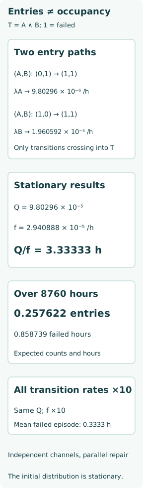
Both components have q = 0.00990099, so Q = qAqB = 0.0000980296, about 0.009803%. This occupancy calculation alone does not identify entries. There are two entering states: A operating with B failed, followed by A failure; or A failed with B operating, followed by B failure.
Count only the transitions that complete the failed combination
The first contribution is λA(1−qA)qB = 9.80296 × 10⁻⁶ h⁻¹. The second is λBqA(1−qB) = 1.960592 × 10⁻⁵ h⁻¹. Their sum gives f_in = 2.940888 × 10⁻⁵ h⁻¹. Simply summing λA and λB would count many single-channel failures that never enter the top event.
From the both-failed state, either repair clears T, so f_out = Q(μA+μB) = the same 2.940888 × 10⁻⁵ h⁻¹. This independent balance check is useful. Multiplying two failure rates would instead produce h⁻² and would not describe an entry frequency. Common-cause transitions, if present, would be additional explicitly modelled paths across the boundary.
Translate the stationary result into episodes and exposure
For an 8760 h observation in stationarity, expected entries are f_in × 8760 = 0.257622, while expected failed time is Q × 8760 = 0.858739 h. A fractional expected count is a population or repeated-observation average, not a partial physical incident. It is not automatically the probability of at least one entry during that year.
The mean failed episode is Q/f_in = 3.33333 h, also 1/(μA+μB) in this model. The mean operating episode is (1−Q)/f_in = 34000 h. The stationary entry intensity conditional on being outside T is f_in/(1−Q) = 2.941176 × 10⁻⁵ h⁻¹. This averaged conditional quantity does not make the aggregated operating-state duration exponential; its internal state history can still matter.
The same unavailability can conceal ten times as many interruptions
For a separate comparison, multiply all four component transition rates by 10. Each ratio λ/(λ+μ) stays the same, so Q remains 0.0000980296. But f_in rises tenfold to 2.940888 × 10⁻⁴ h⁻¹, and the mean failed episode falls to 0.333333 h. Long-run failed hours stay the same while interruptions become more frequent and shorter.
These patterns can have different operating consequences even though an availability summary is identical. A restart penalty, lost batch or transition-induced stress may depend on the count, while lost operating time depends on duration. Neither metric alone fully describes the consequence. The comparison is a time-scaling demonstration, not a maintenance recommendation to increase failure and repair rates together.
With a complemented top event, repair can be an entry transition
Using the same independent component model, consider a different top event H = A ∧ ¬B. One interpretation is a failed barrier A while energy source B is functioning. Entries occur through A failure from the both-operating state and through B repair from the both-failed state. The second is a restoration event at component level but an entry into this specifically defined undesired condition.
Here QH = qA(1−qB) = 0.00980296. The entry contributions are 0.000980296 h⁻¹ from A failure and 0.0000196059 h⁻¹ from B repair, total 0.000999902 h⁻¹. Exit flow is QH(μA+λB), giving the same result. This illustrates why a general boundary-flow calculation checks both failure and repair transitions, and why restoring energy requires the relevant barrier state to be considered.
Report the dynamic assumptions alongside the Boolean logic
Retain the top-event definition, component state meanings, rate units, repair policy, initial distribution, dependencies and observation interval. Show the transitions counted as entries and verify the state balance. If the model begins fully healthy rather than stationary, use transient state probabilities and integrate f_in(t) over the interval for the expected count.
An AND/OR drawing describes combinations, but the frequency calculation needs how those combinations are entered and left. Mission failure probability requires a suitable first-passage calculation; it is not obtained by silently treating entries as a Poisson process. The robust distinction is state occupancy, boundary-crossing count and episode duration, each with its own units and assumptions.