Knowledge / Risk analysis methods
HAZOP of interacting control loops: conflicting actions and disturbed process behaviour
Trace two healthy controllers through a shared mass and energy balance, quantify opposing physical effects, and separate poor tuning from infeasible targets and common equipment failures.
On this page
Two controllers can each act in the correct direction for their own measurement while disturbing the variable controlled by the other. The problem is not necessarily a broken sensor or the wrong sign in a PID block. It can arise from the shared inventory, the energy carried by each stream, or a pair of objectives that the available equipment cannot satisfy together. HAZOP needs to follow those physical effects beyond the controller output labels.
Define the interaction at the process boundary
NPTEL’s multiloop-control lesson describes interaction through inputs that affect both outputs, including effects transmitted through another loop. In this original example, the temperature controller changes hot-feed flow and the level controller changes cold-feed flow into one mixer. The outlet draws from the same inventory. Each manipulated flow therefore affects both the amount of liquid and its thermal state.
The temperature controller opens hot feed when measured temperature is low. The level controller opens cold feed when inventory is low. Both signs are correct for the intended local response. “Controller healthy” consequently does not mean “its action helps every other objective.” A HAZOP node that ends at each valve would miss the shared process through which the actions interact.
Write mass and energy balances before judging the commands
Assume a well-mixed, nonreactive liquid with equal constant specific heat cp and density in both feeds. Hot feed enters at Th = 80 °C, cold feed at Tc = 20 °C, and outlet flow Fo = 2 kg/s leaves at bulk temperature T. There is no external heating, ambient loss, phase change or delay. M denotes the changing mass inventory; no controller dynamics are invented.
MIT’s two-inlet heated-tank lesson provides the mass-and-enthalpy balance framework. For the different variable-inventory mixer here, dM/dt = Fh + Fc − Fo and d(M cp T)/dt = cp(Fh Th + Fc Tc − Fo T). Expanding the left side and substituting the mass balance gives M dT/dt = Fh(Th − T) + Fc(Tc − T). Omitting T dM/dt would produce a wrong temperature equation during filling or draining.
Read the cross-effects at the nominal condition
At M = 100 kg and T = 50 °C, steady operation requires Fh = 1 kg/s and Fc = 1 kg/s. Increasing either inlet increases dM/dt. At that instant the hot-flow effect on dT/dt is (80 − 50)/100 = +0.3 K/kg per unit flow change in kg/s; the cold-flow effect is (20 − 50)/100 = −0.3 K/kg. These are local derivatives of the temperature rate, not steady-state process gains.
Thus a cold-feed action that restores low level initially cools the mixture, opposing temperature recovery. A hot-feed action that restores low temperature also fills the tank. When level later becomes high, closing cold feed reduces filling but also removes a cooling contribution. The signs come from the balances and the current temperatures; they should be reconsidered if a feed temperature crosses the bulk temperature.
Quantify a low-inventory recovery snapshot
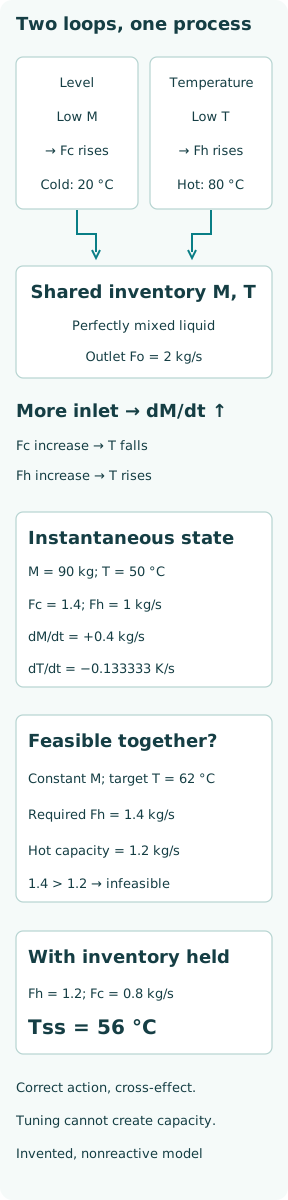
Take a separate instantaneous state M = 90 kg and T = 50 °C. Suppose the level controller has increased cold flow to 1.4 kg/s while hot flow is still 1 kg/s. Mass rises at 1 + 1.4 − 2 = 0.4 kg/s, but temperature initially changes at [1 × 30 + 1.4 × (−30)]/90 = −0.133333 K/s. Level recovery is creating a temperature disturbance even though its valve moves correctly.
If the temperature controller responds by raising hot flow to its stipulated capacity of 1.2 kg/s at that same snapshot state, mass rises at 0.6 kg/s and the temperature rate becomes −0.066667 K/s. Cooling is reduced, but filling is faster. These instantaneous calculations do not predict overshoot or oscillation. That would require the actual controller laws, actuator dynamics and evolving M and T, rather than extrapolating one derivative indefinitely.
Check whether the requested objectives can coexist
Now ask for steady inventory, the same 2 kg/s outlet, and a hypothetical temperature target of 62 °C. The two steady balances require Fh = Fo(Ttarget − Tc)/(Th − Tc) = 2 × 42/60 = 1.4 kg/s and Fc = 0.6 kg/s. The required hot flow exceeds the stipulated 1.2 kg/s capacity by 0.2 kg/s. No choice of tuning gains can create that missing physical capability.
At maximum hot flow with constant inventory, cold flow must be 0.8 kg/s. The corresponding steady temperature is (1.2 × 80 + 0.8 × 20)/2 = 56 °C. Healthy controllers may therefore hold inventory while failing to reach the requested temperature. Persistent temperature error in this condition is evidence to examine target feasibility and capacity before assuming the temperature sensor or controller algorithm has failed.
Show the cost of satisfying only the temperature objective
At hot flow 1.2 kg/s, holding a mixture already at 62 °C requires Fc = 1.2 × (80 − 62)/(62 − 20) = 0.514286 kg/s. That cold flow balances incoming thermal effects, but total inflow is smaller than the fixed outlet. The inventory rate is −0.285714 kg/s. Starting at 100 kg and 62 °C with these constant flows gives M = 82.8571 kg after 60 s, while the ideal temperature remains unchanged.
This is a counterexample, not a suggested way to operate: an apparently successful temperature correction can consume inventory. A level controller trying to replace the deficit adds cold liquid and opposes that temperature hold. The two targets, outlet requirement and hot-capacity constraint must be reconciled at the process-design or supervisory level. Silencing the level loop or bypassing protection would conceal the conflict rather than resolve it.
Distinguish tuning, conflicting objectives and shared failure
A tuning problem concerns the closed-loop response when a feasible operating point exists: excessive interaction, delay or aggressive gains can produce poor recovery. Test that claim with the actual dynamic model and protected response data. Integral windup may worsen a constrained response, but this article’s capacity calculation does not depend on an integrator, and anti-windup cannot make an infeasible target pair feasible.
A conflicting-objective problem is the balance inconsistency just demonstrated. A shared-equipment failure is different again: loss of a common supply, a common measurement error or an incorrectly configured shared actuator can disturb both loops. Diagnose which mechanism is supported by evidence. A trend with two oscillating traces is not enough to distinguish causal interaction, common input disturbance and two separate failures.
Write HAZOP rows around effects and operating modes
For “less inventory,” retain the cold-refill action and its cooling consequence in the row; link it to the temperature-recovery action and the resulting increased filling rate. For “other-than achievable temperature target,” record the capacity constraint, the steady balance that cannot close, and what sustained deviation would mean for the actual process. The hypothetical temperatures alone do not establish a hazardous outcome.
Include automatic/manual transfers, startup, reduced capacity, outlet changes and recovery from a stopped feed. If a supervisory selector or override exists, document its priority and the physical safe state it seeks. A shared valve commanded by two controllers requires explicit arbitration; this example instead uses separate valves and shows that a common process is already enough for interaction. Do not treat the two controller names as evidence of independent protection.
Evaluate coordination without weakening protection
Possible design responses include checking setpoint feasibility before accepting a mode, coordinating inlet ratio and total flow, changing the control pairing, or using a justified supervisory constraint. Which response is suitable depends on the real process and its consequences. The assessment should show how the new structure handles actuator limits, invalid measurements, initialization and return from manual operation.
HSE’s Out of control guidance warns that changes to production control must not degrade overlapping protective functions. Review any common final elements, utilities and signals before modifying the production loops. A coordination improvement is not automatically a new safety layer, and a successful nominal setpoint test does not prove performance when a shared service or final element is unavailable.
Verify the physical response and close the linked rows
On a validated simulator or protected test arrangement, perturb each input separately, observe both process variables, and then test the combined disturbance and relevant mode transitions. Record requested flow, measured flow, actual valve response, inventory, temperature and time. Check whether the observed signs agree with the balance before interpreting controller error or changing tuning.
The closure evidence should identify which mechanism was corrected: a dynamic interaction, an impossible target combination or a demonstrated shared failure. Retain the joint mass and energy calculation with the HAZOP links so a later throughput, feed-temperature or capacity change triggers review. The central finding is that correct local control actions can conflict through the physical process; resolving that conflict requires a feasible combined objective and verified behavior.