Sensor reading control command and physical state

Begin with the quantity being measured

Specify the measurand: the quantity intended to be measured. “Temperature” is incomplete if the distinction between a pipe wall, local fluid, outlet stream and mixed tank matters. Location, time and the physical condition belong to the definition. The JCGM vocabulary entry for measurand explains why this specificity matters.

A sensor interacts with the process. A measurement chain may then condition, convert, transmit, filter and display its signal. An indication is a value provided by that measuring system; it is not automatically an exact process value. See JCGM’s indication entry. A controller and a display may receive different processed versions, so their agreement or disagreement needs context.

Keep five questions separate

1. Physical process: what temperature, flow, pressure, inventory or stored energy exists at the relevant place and time?
2. Measurement: what does the sensing and processing chain report, with what uncertainty, delay and validity?
3. Control command: what action does the controller request, and in which units or defined scale?
4. Actuator response: what movement, rotation or other action actually occurs, and how is it observed?
5. Process response: what change follows in the controlled system after the relevant dynamics and disturbances?

The DOE process-control handbook, IC-07, pages 7–13, distinguishes signal paths, controlled and manipulated variables, and process delays. Signal arrows are not fluid or energy-flow arrows. The Åström–Murray author-maintained introduction explains sensing, computation and actuation as a feedback cycle, including how measurement noise can affect the process through feedback.

Original teaching example with a known bias

All values below are invented. They describe a hypothetical cooler and are neither operating targets nor tuning advice. Let T be its outlet fluid temperature, y the reported temperature, b an introduced measurement offset and n a noise term:

y = T + b + n.

Assume T = 60 °C, b = +3 K and n = 0 at the first instant. The indication is y = 63 °C. Let a purely illustrative reference r = 60 °C define the comparison e = r − y. The controller’s comparison error is −3 K, while r − T = 0 K. The measurement path has created an apparent deviation without an initial physical temperature change.

For this invented cooler, assume a larger controller output requests greater cooling. The biased indication can therefore request more cooling, but the numerical command cannot be calculated without the controller law, its state and limits. An error of −3 K is not itself “70% output.”

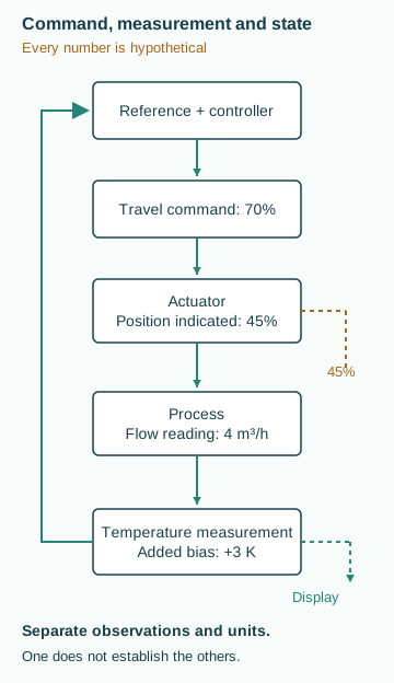
Now stipulate a second hypothetical snapshot: requested valve travel is 70%, position feedback reports 45%, and a separate flow measurement reports 4 m³/h. These are three assigned observations, not values derived from the temperature equation. Seventy percent is the command’s travel scale; 45% is a position indication; neither is 70% or 45% of maximum flow.

The snapshot establishes a command–position disagreement, assuming the scales and timestamps are comparable. It does not establish a stuck valve. Travel may be ongoing, position feedback may be wrong, the command may not have reached the actuator, or the actuator may lack available force. The measured flow adds evidence but has its own uncertainty and depends on hydraulic conditions.

A biased measurement can change the real process

Initially, adding b changes y rather than T. Once the biased measurement affects a functioning feedback loop, the controller and actuator may change actual cooling. Measurement error can then cause a real process deviation.

Suppose, only for this example, the loop reaches a stable feasible equilibrium with y equal to its 60 °C reference, the +3 K bias persists and noise is zero. The model then gives T = y − b = 57 °C. An indication at the reference can coexist with a physical value away from it. This result is conditional: it does not prove that an unspecified controller eliminates its indicated error or that a real cooler reaches that equilibrium.

The signed offset in this model is different from measurement uncertainty. JCGM’s error entry relates error to a measured value and reference value; its uncertainty entry describes the dispersion attributed to the measurand using available information. A displayed reading alone does not reveal its own error. In actual measurements, the exact process value is generally unavailable.

Follow the control and observation layers

The diagram separates the controller’s command, actuator position and process flow. Feedback returns through the measurement chain; the hypothetical +3 K bias belongs to that chain, not to the fluid. The command, indicated position and measured flow are separately assigned observations; neither physical nor statistical independence is assumed.

An accompanying evidence record should retain value, unit, location, timestamp, processing or averaging interval, and whether a value is commanded, measured or inferred. Comparing the layers leaves unresolved explanations visible.

A timestamp is part of the measurement

A value without a reliable time basis can be correct for one instant and misleading for another. Sensor acquisition, communication, filtering and screen refresh can each contribute delay. Two displays labeled with the same wall-clock minute may represent different sample windows. Record whether a timestamp denotes acquisition, processing or receipt, and whether the value is instantaneous or averaged.

For an invented example, suppose the physical temperature rises at a steady 0.2 K per second during a short interval. A reading delayed by five seconds will differ from the contemporaneous value by 1 K even if the sensor has no calibration bias. This is a time-alignment effect under the assumed linear ramp, not proof of a failed sensor. A real transient need not be linear, so the calculation cannot justify correcting every delayed reading by the same amount.

Calibration, adjustment and validation answer different questions

JCGM’s calibration entry distinguishes establishing the relationship between indications and reference values from adjusting an instrument. A calibration record therefore should be read for its conditions, range, uncertainty and result. The word “calibrated” alone does not prove that a measurement is suitable for every installed environment or every downstream decision.

A sensor can behave properly on a bench while measuring the wrong location in service. A correctly scaled transmitter can feed a display that applies the wrong conversion. An instrument can also be accurate over its calibration range but used outside that range. The engineering evidence must follow the installed chain from physical interaction through conversion and processing to the value used by the controller or analyst.

Agreement needs a dependency check

Two matching values are useful only to the extent that their evidence is meaningfully separate. They may share one sensor, one analog-to-digital converter, one power source or one stored value. A second screen displaying the same network message adds visibility, but it does not add a second physical observation. Even physically separate sensors can share an installation error or environmental influence.

In a review, draw the measurement dependencies before describing channels as independent. State whether a comparison uses different principles, locations or signal paths, and whether those differences are appropriate for the measurand. Disagreement between sensors at different locations may represent a real gradient. Agreement after averaging can hide short events. Neither matching nor differing numbers carry a complete diagnosis by themselves.

Data validity should survive the display layer

Missing, stale, out-of-range and substituted values have different meanings. Converting all of them to zero destroys information; silently retaining the last good value can make a changing process look steady. An educational dataset should preserve a validity state, sample age and any substitution policy with the numeric value. The appropriate real-system treatment depends on the approved design and failure response.

A practical analysis record can state: observed value, intended quantity, source path, timestamp basis, processing, validity and unresolved limitations. It should separately state the command and the evidence of actuator and process response. This makes an investigation reproducible without prescribing interlock logic, alarm settings or an unauthorized override. The aim is to avoid claiming more than the observations establish.

Common mistakes and limits

A measurement fault concerns the sensing or reporting function; an actuator fault concerns realizing the requested action. Ordinary measurement noise is not automatically a fault. A steady reading can mean a steady process, filtering or a frozen measurement. A zero reading is not the same as missing data. Two identical display values may come from one shared sensor; agreement then provides no independent confirmation. A moving actuator does not prove the requested flow, and flow does not by itself prove adequate heat removal.

Normal lag is not automatically a fault. Transport time, thermal storage, sampling and actuator dynamics can separate changes in time. Compare like quantities and aligned time windows before interpreting disagreement.

This guide describes public measurement and feedback concepts. It supplies no fault-isolation procedure, protection settings, interlock design or permission to override controls. A real conclusion needs the actual measurement chain, applicable equipment documentation and suitable technical evidence. Sources support the concepts, not the invented case or product claims.

Related guides: Pump curves and system resistance; Cooling-system heat balances; Seawater LT and HT cooling circuits; Verification and validation in physical-system simulation.