Knowledge / Risk analysis methods
Hazard and fragility curves in PSA: from load intensity to failure frequency
Convert exceedance frequencies into disjoint event bins, combine them with conditional fragility, and keep the high-intensity tail visible.
On this page
A hazard curve describes how often a load intensity is exceeded. A fragility curve describes the probability of failure given that intensity. Their product at a convenient point is not generally an annual failure frequency. This original discrete example builds the link carefully, including units, the low-intensity boundary and an explicit upper tail.
Give the two curves different jobs
Let x denote the peak wind speed of one event in m/s, defined at a specified reference location and averaging convention. Let ν(x) be the frequency of events whose peak exceeds x, in year⁻¹. Let g(x) be the dimensionless conditional probability that the selected equipment fails during such an event at intensity x. These quantities answer different questions and have different units.
The hazard curve falls as the threshold increases; fragility often rises as intensity increases. Neither direction alone identifies the dominant risk interval. A frequent weak event can matter through its occurrence frequency, while a rare strong event can matter through its conditional damage probability. The integration has to retain both contributions without counting stronger events repeatedly inside several exceedance thresholds.
Define the event population before calculating
Consider invented wind events affecting a generic coastal service cabinet. Count each meteorological event once by its peak speed. The endpoint is failure of the cabinet’s specified service during that event, not injury, vessel loss or a nuclear damage state. Assume the conditional response has no memory of earlier events and that the event population and equipment configuration remain those described here.
This is an event-frequency model. It does not supply the distribution of the annual maximum wind speed or the probability of at least one annual failure. A conversion between frequency and annual probability requires a counting-process assumption. Consistent event separation, reference height, averaging duration and failure criterion are part of the data definition; incompatible datasets cannot be joined merely because both report wind speed.
List the exceedance values and their units
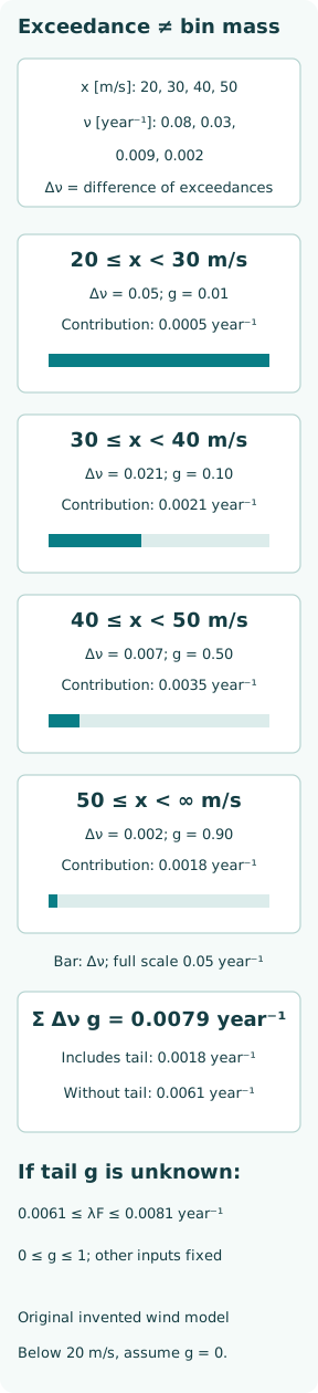
At speed thresholds 20, 30, 40 and 50 m/s, stipulate ν values of 0.08, 0.03, 0.009 and 0.002 year⁻¹. The sequence is non-increasing as required for nested exceedance events. Assume no probability mass exactly on a boundary, so endpoint conventions do not change the numbers. The highest listed threshold is not a claim that stronger events cannot occur.
IAEA’s revised PSA guide connects hazard coverage and site-specific information with conditional fragility. Its context is nuclear safety; no nuclear frequencies or acceptance criteria are borrowed here. For this teaching model, failure probability below 20 m/s is stipulated to be zero. A real lower-bound screening decision would need its own physical evidence rather than this convenience assumption.
Turn overlapping exceedances into disjoint bins
The frequency in [20, 30) m/s is ν(20) − ν(30) = 0.05 year⁻¹. The next two bins have frequencies 0.021 and 0.007 year⁻¹. The open-ended bin [50, infinity) m/s retains 0.002 year⁻¹. These four frequencies sum to 0.08 year⁻¹, matching all events above the lower boundary and preserving the tail.
This subtraction is essential. Every event exceeding 50 m/s also exceeds the lower thresholds, so summing the exceedance frequencies would count it repeatedly. For a differentiable curve, the occurrence-frequency density is −dν/dx, with units year⁻¹ per m/s. ν itself is not that density. For discrete information, finite differences provide the bin masses without inventing a smooth derivative.
Assign event-weighted conditional fragility
Stipulate bin-average failure probabilities of 0.01, 0.10, 0.50 and 0.90 in increasing intensity order. Each value is the conditional average over events in its bin; it is not automatically the fragility at the arithmetic midpoint. Treating fragility as constant within each bin makes this particular discrete model exact for its stated inputs, while remaining an approximation to any unresolved physical response.
The last bin has no finite midpoint. Its 0.90 value is an explicit assumption about the entire tail population. For measured curves, a bin average would weight g(x) by the hazard occurrence measure within that interval. An unweighted average of fragility samples can give the wrong result when events concentrate toward one side of the interval, even if the samples look well spaced.
Integrate and check the failure frequency
Write λF = ∫g(x)[−dν(x)] over the retained intensity range, including its tail. In the bin model this becomes λF = Σ Δνi gi. The four contributions are 0.05 × 0.01 = 0.0005, 0.021 × 0.10 = 0.0021, 0.007 × 0.50 = 0.0035 and 0.002 × 0.90 = 0.0018 year⁻¹. Their sum is 0.0079 year⁻¹.
IAEA’s seismic-evaluation guide describes combining discretized occurrence frequencies with fragility. The mathematical structure transfers here, while its installation-specific inputs do not. The result is nonnegative and no greater than 0.08 year⁻¹ because the conditional probabilities lie between zero and unity. Dividing by that retained event frequency gives 0.09875 failure probability conditional on an event above the lower boundary.
Expose the double-counting shortcut
If the four exceedance frequencies are multiplied by the four bin fragilities and summed directly, the result is 0.0101 year⁻¹. This plausible-looking number is incorrect for the defined model. It assigns the fragility of a lower bin to events that also occupy higher bins, then adds those events again. Matching units is necessary but does not establish correct event accounting.
A useful diagnostic is to replace all bin fragilities conceptually with unity. Correct integration must then return the occurrence frequency of the union of the retained bins, not the sum of nested exceedances. Likewise, a zero fragility everywhere must return zero. Such boundary tests catch errors that a detailed numerical table can hide when its entries are all small and superficially reasonable.
Quantify what the upper tail contributes
Removing the tail leaves 0.0061 year⁻¹. The stipulated tail therefore contributes about 22.8% of the total, despite its low event frequency. A graph cropped at the last finite interval would hide a material part of this example. The largest individual contribution remains the 40–50 m/s bin; the rarest events are not automatically the dominant contribution.
If the tail’s conditional fragility is unknown except that it lies between zero and unity, its contribution is bounded by 0 and 0.002 year⁻¹. The full result is then between 0.0061 and 0.0081 year⁻¹, conditional on the other assumptions. This bound is an uncertainty statement, not a replacement for evidence or a reason to call the truncated result conservative.
Separate resolution from uncertain knowledge
Refining bins tests numerical resolution only when the underlying hazard and fragility information supports that refinement. More rows created by interpolation do not create new evidence. Compare results using justified finer partitions, especially where fragility changes rapidly or hazard mass is concentrated. Check the tail treatment and the lower-bound contribution each time rather than letting them change silently with plotting limits.
Uncertainty in hazard frequency and fragility parameters is a different issue. If they share uncertain physical inputs, their joint treatment may matter; multiplying mean curves can lose that dependence. Document which uncertainty is event-to-event variability and which reflects limited knowledge. Sensitivity cases should preserve the common intensity definition and failure boundary, otherwise an apparent uncertainty range may actually combine incompatible questions.
Keep the load-to-failure chain reproducible
The review package should contain the event definition, intensity reference, exceedance values, bin boundaries, fragility interpretation and endpoint. Record the source and basis of the lower cutoff and tail, including assumptions used where information is sparse. Store each disjoint contribution so that a revised curve can be traced to a changed interval instead of appearing only as a new total.
This calculation does not establish equipment qualification, acceptable maritime risk or a universal environmental design load. It demonstrates a checkable frequency integral for an explicitly invented model. Its practical discipline is to use occurrence mass rather than nested exceedance values, preserve conditional units, and show the parts of the intensity range that are assumed, bounded or left unresolved.