Knowledge / Risk analysis methods
Reliability demonstration tests: sample size, duration and false-acceptance risk
Design fixed mission tests before seeing data, compare zero and allowable failures, and quantify how consumer protection trades against rejecting a good design.
On this page
A successful demonstration is not defined by collecting a pleasing run of successes. Its mission, sample size and acceptance rule must be chosen before the results are known. An original binomial example compares three plans that protect the user at the same reliability boundary but expose the producer to very different rejection risks.
Turn the reliability claim into a repeatable mission
Define success as completing a specified 20 h sensor mission within its functional limits under a stated environmental and load profile. Each independently sampled unit receives one complete mission. Let r be the common probability of success and X the number of failed missions among n units. Under the sampling assumptions, X follows a binomial distribution with failure probability 1 − r.
The mission definition must include the failure criteria, measurements, preparation and treatment of an incomplete trial. A unit that was never exposed to the required load has not supplied a successful mission. The illustrative plans concern this narrowly defined success probability. They do not automatically demonstrate an annual fleet reliability, a longer mission or performance under a different environment.
Specify both sides of the decision error
Call rB = 0.95 the unacceptable boundary and require the probability of accepting any r ≤ rB to be no greater than 0.10. Separately call rG = 0.99 the good-design point and target a rejection probability no greater than 0.10 there. The interval between the two reliability points is deliberate: a finite test cannot sharply separate nearly identical performance with no errors.
NIST’s binary-threshold guidance treats false acceptance and false rejection as design quantities. Here consumer risk means accepting the bad boundary; producer risk means rejecting the good point. These verbal definitions matter more than a bare Greek letter because type-error labels depend on which hypothesis is written as the null. Every displayed risk below uses the stated definitions.
Write the fixed acceptance rule and its probability
A plan (n, c) accepts if X ≤ c after the n specified missions. Its operating-characteristic probability is Paccept(r) = Σⱼ₌₀ᶜ C(n,j)(1 − r)ʲ rⁿ⁻ʲ. NIST’s sampling-plan treatment uses this binomial sum and two designated quality points. The present application is mission reliability rather than a claim about a particular manufacturing lot.
For fixed n and c, acceptance becomes more likely as r increases. Consequently the worst acceptance probability over r ≤ 0.95 occurs at 0.95. This monotonicity is why checking the boundary controls the entire lower-reliability region under the model. It does not cover a biased sample, dependence or a mission definition that excludes relevant failures.
Calculate the zero-failure plan first
With c = 0, Paccept(r) = rⁿ. Requiring 0.95ⁿ ≤ 0.10 gives n ≥ ln(0.10)/ln(0.95), so the smallest integer sample is 45. Its boundary acceptance probability is 0.099440. With 44 missions it would be 0.104674, above the chosen consumer-risk limit. Rounding sample size downward would therefore change the promised test property.
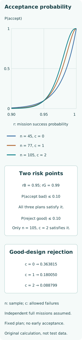
At the good point r = 0.99, the 45-mission plan accepts with probability 0.636185 and rejects with probability 0.363815. Zero tolerated failures sounds demanding, but it is costly for a genuinely good design because a single ordinary failure rejects the entire test. This plan meets the consumer-risk target and fails the producer-risk target in the original example.
Allow failures while preserving consumer protection
For c = 1, the smallest sample meeting the consumer target is n = 77. For c = 2, it is n = 105. The table compares the resulting plans at the same two reliability points; all probabilities are rounded to six decimals. Increasing the failure allowance without increasing sample size would not preserve the same boundary protection.
| n | c | Accept, r = 0.95 | Reject, r = 0.99 |
|---|---|---|---|
| 45 | 0 | 0.099440 | 0.363815 |
| 77 | 1 | 0.097327 | 0.180050 |
| 105 | 2 | 0.099187 | 0.088799 |
The two-failure plan accepts the good design with probability 0.911201, so its rejection probability is 0.088799. It meets both selected risk limits. The one-failure plan’s good-design acceptance is 0.819950, leaving too much producer risk for the stated target. The plans are original computed examples, not recommended acceptance criteria for every component or safety function.
Interpret a passing result as a bounded confidence statement
If all 45 missions succeed under the fixed zero-failure plan, exact binomial inversion gives the one-sided 90% lower confidence bound rL = 0.10^(1/45) = 0.950119. Exact binomial limits avoid a misleading normal approximation near an all-success sample. A passing result supports the stated boundary at the specified confidence level under the sampling model.
This is not a 90% posterior probability that r exceeds the boundary, nor does it mean that the tested units cannot fail later. For an allowable-failure plan the bound must use the actual observed count, not the zero-failure formula. Inverting the binomial tail at the prespecified allowance gives the corresponding limiting acceptance boundary; fewer observed failures provide stronger evidence within the same fixed design.
Budget unit exposure and calendar duration separately
At 20 h per complete mission, the planned slot totals are 900 h for n = 45, 1540 h for n = 77 and 2100 h for n = 105. These are unit-hours, not wall-clock test durations. With five synchronized stations and full-length slots, the corresponding calendar allocations are 180 h, 320 h and 420 h before setup, interruptions and reporting.
Parallelization does not by itself create independent evidence. A shared chamber excursion, power interruption or preparation batch can correlate outcomes. Nor can one long run automatically be split into independent missions: accumulated damage and unit-specific frailty can carry across artificial boundaries. If repeated trials on the same units are intended, justify a suitable model and redesign the risk calculation rather than simply counting more trials.
Freeze the stopping and retest rules before starting
Under a fixed plan, early rejection after more than c failures is logically consistent because later successes cannot reverse that final decision. Early acceptance after a favorable partial sequence is a different rule and generally has a different error probability. A formally designed sequential plan can be valid, but its boundaries and analysis must be established as that plan.
A failure followed by repair and an unplanned restart cannot quietly erase the first result. Decide beforehand how invalid tests, laboratory faults, configuration changes and corrective actions will be classified. If a redesigned product is tested anew, preserve the earlier evidence and state the new population. Repeatedly launching fresh demonstrations until one passes changes the probability of eventual acceptance.
Protect the evidence with sampling and configuration control
Select units that represent the intended production and operating population. Keep environmental coverage, manufacturing variation and software or hardware configuration visible. Choosing only the best laboratory units changes the target population even if the binomial arithmetic is perfect. A demonstrated mission criterion also needs adequate measurement sensitivity; undetected failures count as apparent successes in the recorded data.
Record all prespecified missions, their outcomes and reasons for exclusions. If a common cause affects several units, investigate it as a physical mechanism and as a violation of the independent-trial model. A larger nominal n cannot guarantee the advertised risk when the effective information is dominated by a few shared conditions. The statistical design and the engineering test procedure must describe the same experiment.
Choose the plan for the decision it must support
The two-failure plan buys a much lower chance of rejecting the good point with more units and test time. That is the central tradeoff in this case, not a general rule that more allowable failures are always better. Costs, destructive testing, required reliability and acceptable error probabilities determine which plans are feasible; any compulsory qualification requirements remain separate constraints.
A reviewable plan contains the mission, population, two risk points, fixed n and c, duration, independence rationale and stopping rules. After testing, report the actual counts, confidence calculation and deviations against that record. This keeps a demonstration from becoming a retrospective search for a favorable number and makes clear exactly which reliability claim the experiment can support.