Knowledge / Risk analysis methods
Partial pooling in fleet reliability: shared information and unit-specific differences
Compare matched-prior separate, complete and hierarchical pooling for three fictional fleet groups, keeping hyperparameter uncertainty and new-group prediction explicit.
On this page
A fleet may contain many similar units but little evidence for each one. Treating every unit as unrelated wastes potentially relevant information; assigning one probability to the whole fleet erases differences. This original three-group example shows exactly how a shared population model lets groups inform one another while preserving separate failure probabilities.
Define comparable demands and the exchangeable population
Let pj be the probability that a unit in group j fails a specified demand. The demand definition includes the required function, duration and operating conditions. Group counts can be pooled only after checking that their denominators refer to comparable opportunities. A start attempt, an hour of operation and a completed voyage are different evidence units and cannot share a binomial denominator merely because each has a failure label.
Exchangeability means that before observing the outcomes, permuting group labels within the stated population does not change the joint probability model. It does not mean the groups have identical probabilities or identical equipment histories. If temperature, configuration or duty distinguishes groups in a relevant way, condition on those features, model them as predictors or separate the populations before borrowing information.
Keep the original group evidence visible
Use fictional failure counts A: 1/20 demands, B: 0/5 and C: 5/25. The pooled empirical fraction is 6/50 = 0.12, but that number neither proves equality of group probabilities nor establishes perfection for B. These deliberately small counts illustrate an inference problem; they are not observations from a vessel, operator or supplier.
Hierarchical partial pooling models a population of group probabilities and learns its properties from the groups. Complete pooling uses one common probability. No pooling keeps the group analyses independent. Partial pooling shares population information while retaining pj for each group. To make the comparison below interpretable, all three models start with the same marginal prior distribution for an individual probability.
Specify a real hierarchy rather than a fixed fleet prior
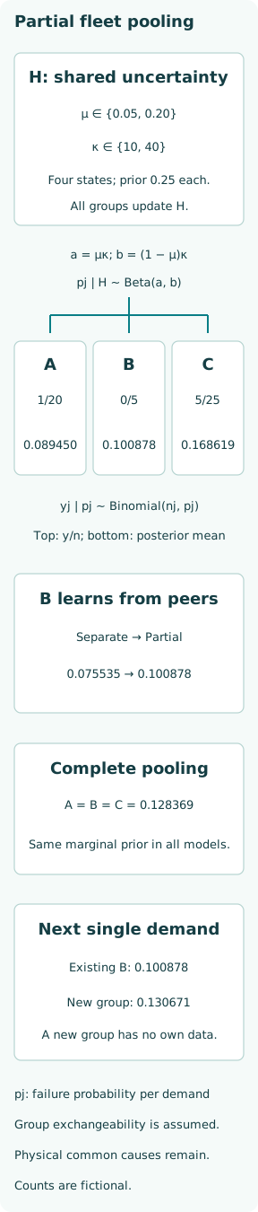
Let the shared hyperparameter state H choose a pair (μ, κ). Conditional on H, pj follows Beta(μκ, (1 − μ)κ), independently across groups. Then yj conditional on pj follows Binomial(nj, pj). Here μ is the population mean failure probability and κ controls concentration; the conditional population variance is μ(1 − μ)/(κ + 1). All probabilities and these shape parameters are dimensionless.
For an auditable small calculation, use four equally likely hyperparameter states: μ can be 0.05 or 0.20, and κ can be 10 or 40. This is a fully specified discrete hyperprior, not a claim that the true fleet can have only those properties. Both the population mean and concentration remain uncertain and are updated by all group likelihoods. Fixing them after looking at the data would discard part of this hierarchy.
Update the shared population distribution from every group
For state h, put ah = μhκh and bh = (1 − μh)κh. Its marginal group likelihood is C(nj,yj) B(ah + yj, bh + nj − yj)/B(ah,bh), where B is the beta function. This beta-binomial mass results from integrating out the group probability. Multiply those likelihoods across groups and by the state’s prior weight, then normalize across states.
| H | μ | κ | Prior | Posterior |
|---|---|---|---|---|
| H1 | 0.05 | 10 | 0.25 | 0.228168 |
| H2 | 0.05 | 40 | 0.25 | 0.234026 |
| H3 | 0.20 | 10 | 0.25 | 0.286612 |
| H4 | 0.20 | 40 | 0.25 | 0.251194 |
The resulting weights are spread across all four states; the small sample has not selected a single known population. Binomial coefficients can cancel when comparing these states because they are constant with respect to h. They remain part of a normalized count distribution when computing predictive probabilities. The shared update is what transfers information between groups without forcing their pj values to coincide.
See the shrinkage inside each conditional posterior
Conditional on a particular h and the data, pj has distribution Beta(ah + yj, bh + nj − yj). Its mean is (yj + κhμh)/(nj + κh), a weighted average of the group’s empirical fraction and μh. The data weight is nj/(nj + κh); the population weight is κh/(nj + κh). Sparse groups receive more population influence at the same κh.
The full posterior mean averages that expression over the updated weights of H. It is not obtained by inserting a single guessed fleet mean or by reusing the total failure count inside every group likelihood. Group data contribute once to the joint hierarchy. In this example the posterior means are 0.089450 for A, 0.100878 for B and 0.168619 for C. Their separation survives the borrowing.
Compare pooling choices with matched marginal priors
For no pooling, each group receives its own independent hyperparameter state drawn from the same four-state prior and updates it using only its own counts. For complete pooling, a single p with that same marginal beta-mixture prior receives all 6 failures in 50 demands. This controls the prior marginal while changing how probabilities are related across groups.
| Group | y/n | Separate | Partial | Complete |
|---|---|---|---|---|
| A | 1/20 | 0.071221 | 0.089450 | 0.128369 |
| B | 0/5 | 0.075535 | 0.100878 | 0.128369 |
| C | 5/25 | 0.190629 | 0.168619 | 0.128369 |
Partial pooling raises the separate estimates for A and B and lowers C here. It does not pull every estimate to the empirical fleet fraction or to a universal fixed target. The complete-pooling posterior mean is identical for all groups, while the separate model cannot let C’s failures inform B. The table reports means only; a decision sensitive to uncertainty needs the full posterior mixtures or their derived intervals.
Predict existing and new groups differently
For B’s next single demand, the posterior failure probability is its mean 0.100878. A previously unobserved exchangeable group instead draws a fresh p from the population model, giving next-demand failure probability 0.130671. B’s own successful demands inform its existing group probability; a new group has no such history. Using B’s posterior for an unobserved group would borrow evidence at the wrong level.
For five future demands within one group, integrate the group probability before reporting at least one failure. The result is 0.364183 for existing B and 0.432254 for a new group. In each beta component the no-failure probability is B(a, b + 5)/B(a,b), using updated a,b for B and population a,b for the new group, then averaging over H. Substituting B’s mean into a binomial formula instead gives 0.412386 and loses uncertainty.
Preserve operational differences and common-cause pathways
Sharing a population distribution is not a repair for unlike service conditions. If C operates in a harsher environment, shrinking it toward calmer groups without a relevant predictor can conceal a real mechanism. Keep covariates and configuration changes in the evidence record. A group with many demands can dominate a poorly specified model while its operational difference remains hidden behind a plausible fleet average.
Conditional independence also needs its own engineering basis. Uncertainty in shared H creates predictive association between groups, but that association is not a physical common-shock model. Contaminated fuel, common software or one power interruption can jointly affect demands beyond the assumed hierarchy. Pooling does not remove those common causes; model their event structure or clustered likelihood separately when the data and decision require it.
Check what the hierarchy predicts, including its weak points
Predictive checks compare model-generated outcomes with relevant data features and distinguish existing from new groups. Examine whether the model can reproduce groups with no failures, the spread of group fractions and unusual clusters. Assess new-group forecasts by holding out whole groups, not only isolated demands from groups whose histories already informed the fit. Use the same operational target as the intended forecast.
As a sensitivity illustration, omitting B’s data moves the predicted new-group mean from 0.130671 to 0.157001. That is a model recalculation, not a validation result or permission to delete favorable evidence. With few groups, hyperprior choices remain influential. Expand or vary the finite support and prior weights, inspect the resulting predictions and disclose changes that would alter the engineering decision.
Carry a distribution and a population definition into the decision
The hierarchy produces estimates for known groups and forecasts for new comparable groups, with uncertainty in both group probabilities and population properties. It does not certify a fleet, correct missing demand records or identify a causal reason for C’s higher count. A decision about one vessel must preserve that vessel’s relevant conditions rather than inherit an undifferentiated fleet number.
Retain the group counts, exchangeability rationale, full hyperprior, likelihood, posterior state weights and predictive target. The exact finite calculation makes information sharing inspectable: the population learns from the groups, and each group retains its own evidence. Its usefulness ends where the population definition or conditional independence assumptions cease to fit the physical fleet.