Knowledge / Risk analysis methods
Latent multiple faults in FMEA: from single-fault review to combination checks
Follow a hidden shutdown failure and a later control failure through an original four-state matrix, then calculate a bounded exposure example and decide when FTA or a state model is needed.
On this page
A protective function can be unavailable while the equipment still appears to operate normally. A later operating failure then encounters a system that has already lost its intended protection. Reviewing each failure only against an otherwise healthy system can conceal this interaction. A combination check makes the changed starting state visible; it does not turn an FMEA worksheet into a probability model.
Identify the assumption inside a single-failure row
NASA GSFC-HDBK-8004 describes failure-mode analysis as examining one mode at a time and distinguishes individual modes from event sequences. That is a useful boundary, not evidence that simultaneous or sequential failures are impossible. A row saying “backup shutdown prevents overheating” contains an important condition: that shutdown must still be available when demanded.
Preserve the ordinary single-failure rows, then ask which credited functions can fail without an immediate visible effect. Connect those hidden modes to the initiating faults whose consequences they change. This exercise concerns the interaction between failures; increasing or decreasing a detection score alone does not establish what happens in the combined state.
Define two faults and one physical outcome
Consider an illustrative electrically heated service tank. The primary control contactor regulates heating. A separate high-temperature shutdown path can interrupt power and latch the heater off. D means the primary contactor remains closed when heating should stop. L means the shutdown path has already developed a hidden inability to interrupt power. Normal temperature regulation does not exercise that interrupting function fully.
Define H as continued heating beyond a stated unacceptable temperature limit following D. Assume sustained heat input is sufficient to cross that limit, the healthy shutdown acts early enough to prevent H, the failed path cannot interrupt, and no other protective action intervenes. These are teaching assumptions, not a real tank design assessment. Heat input, stored heat, sensor location, trip delay and the isolation device would need physical verification before assigning the same outcomes to equipment.
Read all four cells of the combination matrix
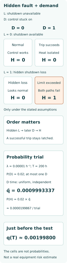
With L = 0 and D = 0, regulation continues and shutdown remains available. With L = 0 and D = 1, normal control is lost, but the shutdown interrupts heating before the limit. The second state is an abnormal shutdown, not normal availability, even though H is prevented.
With L = 1 and D = 0, the tank may look normal because the primary contactor still regulates it; protection has silently disappeared. With L = 1 and D = 1, neither path stops heating and H occurs under the defined boundary. The compact logical condition is H = L AND D, where L is evaluated when D demands protection. The matrix describes consequences, not cell probabilities.
Make the hidden interval and the order visible
The important path is healthy operation → hidden shutdown loss → primary-control failure → H. The exposure interval begins when the shutdown capability is lost, not when a maintenance record eventually reports it. A routine display of normal tank temperature does not prove that the shutdown path could open under a demand.
Reverse the order and the history can change: if D occurs while shutdown is healthy, the assumed latching isolation removes heat. A later inability to open does not by itself reconnect an already isolated heater. Restart, bypass, reclosure or a failure during the trip would require additional events. A Boolean AND drawn without time or state definitions can blur these different histories.
Set up a probability trial separately from the FMEA
Use an original hypothetical trial lasting one T = 200 h test interval, beginning with the shutdown path working. Let its time to the specified hidden failure be exponential with constant rate λ = 0.00001 h⁻¹. It remains undetected and unrepaired until a test or a demand reveals it. At the scheduled test, assume perfect detection and immediate restoration, with no test downtime or repair delay.
Stipulate that the trial contains either no D or exactly one D, with P(D) = 0.02. If D occurs, its time is uniformly distributed across the interval and independent of the shutdown-path lifetime. This explicitly specified one-demand model is not an exponential failure model for the primary contactor. Assume a healthy shutdown always completes successfully; omit other protections, common causes and demand-induced failures. None of these inputs is inferred from an FMEA ranking.
Calculate the combined probability from exposure
The NRC Fault Tree Handbook relates periodic testing of hidden standby failures to an interval-average unavailability and states the uniform-demand and perfect-test assumptions. For the trial just defined, at time t the chance that L has already occurred is q(t) = 1 − exp(−λt). Averaging the independently timed demand gives q̄ = [integral from 0 to T of q(t) dt]/T = 1 − [1 − exp(−λT)]/(λT).
Here λT = 0.002 and q̄ = 0.0009993337, about 0.099933%. Thus P(H) = P(D) × P(L present when D occurs | D) = 0.02 × q̄ = 0.0000199867 per trial. The small-λT approximation q̄ ≈ λT/2 gives 0.001 and P(H) ≈ 0.00002. It overestimates this exact trial result by about 0.06668%. These are dimensionless probabilities for the stated experiment, not events per hour or measured accident rates.
Do not replace the average with the end-of-interval value
Immediately before the 200 h test, q(T) = 1 − exp(−0.002) = 0.0019980013, almost twice the interval average. This is the relevant conditional unavailability for a demand just before the test. It is not interchangeable with the value for a demand uniformly distributed between tests. If operating upsets cluster near a particular test age, replace the uniform weighting with the justified demand-time distribution.
For comparison, a 100 h test interval gives q̄ = 0.0004998334 for the same latent rate and a uniformly timed demand, roughly halving conditional unavailability. That does not establish a real maintenance interval or halve annual accident probability. The frequency of initiating faults, incomplete test coverage, downtime and maintenance-induced faults are absent from this calculation; P(D) has not been respecified for a 100 h trial.
Choose the next model and challenge independence
FAA AC 25.1309-1B identifies FMEA as a source for fault-tree events and describes state models for more complex transitions. Use an FTA to assemble other sufficient combinations leading to the defined outcome. Use a state or sequence model when latching, detection, repair, restart or event order changes the available paths. A fixed periodic-test schedule should not silently become an exponential repair transition merely because a continuous-time Markov tool is convenient.
The product above is justified only by the trial’s independence assumptions. A common supply fault, shared sensor error or maintenance mistake might affect both control and shutdown. In that case use the appropriate conditional probability or an explicit common-cause event; do not multiply marginal probabilities and call the two paths independent because their component names differ. The cited aerospace and nuclear methods provide analytical context, not maritime certification limits.
Turn the four cells into a controlled verification plan
On a safe simulator or suitably protected test rig, establish normal regulation, inject D with shutdown available, represent L alone, and then apply D while L is already present. Check the physical isolation response and the state reached, not only whether a software alarm or relay command appeared. The combined case verifies the analysis boundary; it must not expose an operating tank to an actual hazardous temperature.
Also test the proof-test procedure against the specific L mechanism. A lamp test or simulated sensor input can leave the final power-interrupting device untested. Record which chain elements were exercised, the maximum interval before this mode can be discovered, and what happens after a failed test. Include restored wiring, removed bypasses and a verified return to service. A nominal test frequency is not evidence of detection or successful restoration.
Close the loop without losing the two original rows
Keep each single-failure row’s identifier, immediate effect and detection method. Add the affected protective function, the hidden state it can create, the other row that makes that state consequential, and the combination-model reference. If L is assumed present, D has a different system effect; retaining that conditional consequence prevents the original “protected” assessment from being reused without its prerequisite.
Closure requires evidence for the control that actually breaks the sequence: a design change, a demonstrated functional test, a bounded restoration process or a justified operating restriction. Assign an owner and revisit the linked rows when the contactor, shutdown logic, test method or interval changes. The useful result is a traceable account of which second fault becomes dangerous after a hidden first fault, together with verified measures and an explicit record of what remains outside the model.