Knowledge / Risk analysis methods
Competing failure mechanisms: cause-specific hazard and cumulative incidence
Distinguish a mechanism’s hazard among working units from its share of first failures, and see why reducing one mode can increase another mode’s observed incidence.
On this page
A module can stop working because its seal fails or because its electronics fail. The first failure ends that module’s service record, so the second mechanism loses the opportunity to appear as its first failure. An original two-mechanism example shows why mechanism-specific life, total survival and observed mode incidence answer different questions.
Define the first-failure endpoint and the clock
Follow new modules from installation until the first loss of the specified function. Let T be that first-failure time in operating hours and J identify its diagnosed cause, A or B. A is seal-related loss and B is electronics-related loss. These labels are fictional engineering categories, not measured rates or a claim that every real component has only these mechanisms.
Specify what counts as function loss, how ambiguous diagnoses are handled and whether dormant calendar aging occurs outside the operating-hour clock. A later workshop discovery of both damaged parts does not automatically establish which failed first. If failures can occur simultaneously from one shock, the endpoint set needs a joint-cause state or a justified attribution rule; silently forcing every event into A or B changes the question.
Keep the survivor population in the hazard definition
The cause-specific hazard hA(t) describes the instantaneous rate of an A first failure among modules still free of every counted failure just before t. It has units of inverse hours. The cumulative incidence FA(t) = P(T ≤ t, J = A) instead uses the original installed population and is dimensionless. A rate among survivors is not a fraction of all installed units.
With continuous event times and exhaustive mutually exclusive first-failure causes, h(t) = hA(t) + hB(t). Overall survival is S(t) = exp[−∫₀ᵗ h(u) du]. These identities use the observed first-event process; they do not require independent hypothetical times for each mechanism. They do require a coherent risk set and a shared endpoint definition. Ordinary end-of-study censoring adds separate estimation assumptions when fitting data.
State the extra assumption behind a product construction
A latent lifetime TA describes when A would fail if the competing endpoint did not stop observation; TB is defined analogously. If these latent lifetimes are independent and the module fails at their minimum, S(t) = SA(t) SB(t). NIST’s competing-risk construction explicitly uses independence, first-mechanism failure and known mode distributions. Those assumptions make a mechanism-by-mechanism model possible.
Independence is stronger than merely recording distinct cause names. A high-temperature environment could speed both mechanisms, making unconditional lifetimes dependent even if they are independent at a specified temperature. First-failure observations alone generally do not identify the joint distribution of unobserved latent lifetimes. Multiplying separate marginal survival curves therefore needs a physical and statistical argument beyond the availability of two fitted curves.
Build a transparent constant-rate example
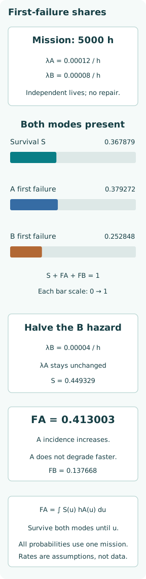
Assume independent exponential latent lifetimes with λA = 0.00012/h and λB = 0.00008/h throughout an original 5000 h mission. Both rates are invented for this demonstration. There is no repair or replacement within the mission. The exponential model has survival exp(−λt) and constant hazard; here its use is a deliberately limited simplification, not an assertion about seal aging.
The total hazard is 0.00020/h, so S(5000) = exp(−1) = 0.367879 and the probability of any first failure is 0.632121, rounded to six decimals. Multiplying the rate by time gives cumulative hazard, not the exact failure probability. In this example the cumulative hazard equals unity, making the difference too large to hide behind a rare-event approximation.
Integrate the hazard against overall survival
The cumulative-incidence construction weights each cause’s hazard by overall event-free survival: FA(t) = ∫₀ᵗ S(u) hA(u) du. For the constant-rate example this becomes FA(t) = [λA/(λA + λB)] [1 − exp(−(λA + λB)t)]. FB uses the same denominator and survival factor with λB in the numerator.
At 5000 h, FA = 0.379272 and FB = 0.252848. The exact unrounded values satisfy S + FA + FB = 1. The mode fractions among all first failures are 0.6 and 0.4 here only because the hazards maintain a constant ratio. If their time shapes differ, that fraction can change with the reporting horizon, so a single failure-mode percentage is not generally transportable between missions.
Compare incidence with a mechanism’s net failure probability
If B were absent while A’s lifetime law stayed unchanged, the A failure probability at 5000 h would be 1 − exp(−0.00012 × 5000) = 0.451188. The analogous net B probability is 0.329680. These are not the observed first-failure incidences 0.379272 and 0.252848 when both mechanisms compete. Adding the two net probabilities does not partition the first-failure population.
The difference is opportunity: some modules that could eventually fail through A have already failed through B. Calling the larger net quantity “A risk in the current fleet” overstates that observed incidence. Conversely, describing the smaller incidence as proof of a more durable seal confuses the seal mechanism with removal of units by another failure mode. Name the estimand before comparing numbers.
Check the apparent reversal after improving another mode
Halve λB to 0.00004/h while keeping λA unchanged. Overall survival at 5000 h rises to 0.449329. A incidence nevertheless rises to 0.413003, while B incidence falls to 0.137668. More modules remain available to experience A before the mission ends. The increased A incidence is compatible with unchanged A hazard and improved total reliability.
If B is entirely removed under the stronger unchanged-A assumption, survival becomes 0.548812 and A incidence becomes 0.451188. This is a model counterfactual, not an identified causal effect of any particular redesign. A real electronics modification might also change enclosure heat, sealing, operating duty or diagnostic classification. Those pathways must be checked before reusing the counterfactual values as an engineering forecast.
Treat competing events and censoring according to the target
For fitting an observed cause-specific hazard, a B event removes the module from the A risk set at that event time. That bookkeeping does not make B ordinary independent loss to follow-up. Converting an A-only survival fit into one minus survival estimates a net construction, not automatically the fleet’s observed A incidence. The distinction survives even when a software interface calls both removals “censored.”
For absolute first-cause probabilities, retain all competing endpoints and use a compatible cumulative-incidence or multi-state calculation. Administrative study closure requires noninformative censoring, possibly conditional on recorded covariates; preventive removal driven by suspected deterioration may violate it. Unknown causes also need explicit treatment. A convenient diagnosis code is not a substitute for evidence that the missing classifications are harmless.
Keep rate, fraction and consequence separate
An A first failure need not have the same consequence as a B first failure. A mode-incidence calculation describes which defined failure appears first; it does not by itself supply severity, recovery success or downstream damage. If those outcomes matter, attach them with compatible conditional models and preserve the initial cause and exposure basis. Do not multiply by a mode fraction already embedded in the cause-specific rate.
Likewise, this nonrepairable mission model does not estimate repeated failure counts or stationary availability for a repaired fleet. Replacement restarts a new life only under an appropriate renewal assumption, and imperfect repair can preserve aging or latent damage. Report the population, horizon, diagnostic rules and model assumptions alongside the incidence values so another analyst can tell which of these extensions is absent.
Use the result to frame a defensible comparison
Compare design alternatives with total survival and all relevant cause incidences on the same mission. Investigate whether a falling mode share reflects a lower cause hazard or a more aggressive competing mode. Preserve uncertainty in both hazards and their dependence structure; more digits in the displayed incidence cannot compensate for sparse diagnoses or an untested independence claim.
The numerical check is simple: probabilities must be nonnegative, incidence must start at zero, and survival plus the complete set of first-cause incidences must sum to unity. The engineering check is harder: the endpoint set, clock and latent-mechanism assumptions must remain defensible. Together those checks stop a useful mode model from quietly answering a different reliability question.