Pump curves and system resistance

Start with head and flow

Volumetric flow Q describes volume transported per time, commonly m³/s or m³/h. Pump head H describes added mechanical energy per unit weight and is expressed in metres of the pumped liquid. It is not simply the vertical height of a pipe or a pressure reading at one point.

For an incompressible liquid, the pressure contribution to a head difference is Δp/(ρg). A full head comparison may also include elevation and velocity terms. Thus converting head to pressure requires density, and comparing suction and discharge measurements requires consistent locations and reference conventions. DOE’s fluid-flow handbook, HT-03, develops the energy and head-loss relationships.

A manufacturer’s pump curve applies to specified conditions, including speed and impeller configuration. The associated efficiency, power, suction requirements and permissible range are additional information. A curve intersection by itself is not evidence that a pump is suitable.

What the system curve represents

The system requires head to overcome static differences and flow-dependent losses. A useful teaching approximation is H_system = H_static + KQ², with K expressed in units consistent with Q. It is not a universal law. Friction factors, fluid properties, flow regime, component behavior and network configuration can change the curve.

Static head can include an elevation difference or a pressure difference between boundary reservoirs. In a completely filled closed circulation loop returning to the same state and elevation, elevation changes around the loop cancel; the pump still supplies the head needed for losses. Simply adding every upward pipe section invents a static requirement.

KSB’s system-characteristic explanation separates static terms from flow-dependent losses and states the assumptions behind a quadratic loss relationship. Its operating-point explanation shows why either curve changing can move the intersection.

Original worked example

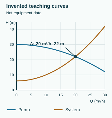
The following curves are invented for teaching. They are not measured, certified or associated with any pump model. Assume steady, single-phase water flow, one simple flow path and a fixed pump speed. Use the curves only over the illustrative flow range 0–30 m³/h.

Define q = Q/(1 m³/h), so q is a dimensionless numerical flow coordinate. Then:

• Pump curve: H_pump = (30 − 0.02q²) m
• Initial system curve: H_system = (6 + 0.04q²) m

Writing q explicitly prevents a common unit error: these numerical coefficients cannot be reused unchanged with Q expressed in m³/s.

At the intersection, 30 − 0.02q² = 6 + 0.04q². Therefore 24 = 0.06q², q² = 400, and the positive-flow solution is Q = 20 m³/h. Substitution into either curve gives H = 22 m.

The plotted intersection A is Q = 20 m³/h and H = 22 m. The zero-flow intercept is a mathematical reference, not an instruction to operate at zero flow.

Change resistance while holding the pump curve fixed

Now introduce a second invented system curve, H_system,2 = (6 + 0.08q²) m. This represents greater flow-dependent resistance while leaving the static term unchanged. It does not identify the physical cause.

Equating curves gives 24 = 0.10q². The new intersection B is Q = √240 = 15.49 m³/h and H = 25.20 m. Check the result on both sides: the pump gives 30 − 4.8 = 25.2 m, while the system needs 6 + 19.2 = 25.2 m.

Flow decreased by about 22.5%, even though the pump curve stayed the same. Head increased. A higher indicated pressure difference can therefore coexist with reduced flow in this teaching case. It is not a general diagnosis of blockage; different curve shapes and boundary changes can produce other results.

Inputs are the two curve equations, their units, the modeled configuration and fluid assumptions. Outputs are paired flow and head values. Neither “running” nor “more pressure” is a substitute for that pair.

Two pumps still need a system curve

For idealized parallel pumps connected between the same hydraulic nodes, add individual flows at a common head. For series pumps without an intervening branch, add heads at a common flow. KSB’s series-operation reference explains the latter construction. These additions create combined curves; they do not fix the resulting system flow.

For two identical copies of the invented pump in ideal parallel connection, each carries half the total flow. The combined curve is H = (30 − 0.005q_total²) m. Against the original system, 24 = 0.045q_total², giving 23.09 m³/h total at 27.33 m. This is more than 20 m³/h but far below 40 m³/h. The network’s rising head requirement explains the difference. Branch losses and unequal pumps would require a fuller model.

Power is another question

With assumed density 1000 kg/m³ and g = 9.81 m/s², the initial point delivers hydraulic power ρgQH = [1000 × 9.81 × (20/3600) × 22] W = 1199 W ≈ 1.20 kW. This is power transferred to the liquid. Shaft input is larger when pump efficiency is below one; electrical input also depends on motor and drive losses. No efficiency or motor rating has been established here.

A valid intersection still needs a suction check

A head–flow intersection assumes the pump can operate there with the supplied liquid. Available suction conditions and the manufacturer’s required net positive suction head must also be assessed on compatible reference and test bases. NPSH concerns the inlet energy margin above vapor pressure, not simply the discharge pressure. Higher liquid temperature changes vapor pressure; suction losses and source level can change the available margin.

KSB’s cavitation explanation distinguishes cavitation criteria, including a specified head-drop criterion. Meeting a quoted NPSH value must therefore be interpreted with its definition and the required design margin; it does not automatically mean all cavitation effects are absent. This article gives no universal margin. A real assessment uses the applicable pump data and system conditions, including the least favorable approved operating cases.

A speed change moves both the question and the evidence

For geometrically unchanged pump operation within a suitable similarity regime, KSB’s affinity relationships relate flow to rotational speed, head to speed squared and power to speed cubed at corresponding points. These are scaling relationships with assumptions, not a guarantee that actual system flow follows speed linearly. The new pump curve must still be intersected with the actual system curve, especially when a static term is significant.

An original illustration uses the article’s invented pump curve. At 80% of its original speed, ideal similarity gives H = 19.2 − 0.02q² metres. Against the original system curve, 19.2 − 0.02q² = 6 + 0.04q², yielding q = √220 = 14.83 and head 14.8 m. Actual modeled flow is about 74% of the original 20 m³/h, rather than 80%, because the static term remains. The arithmetic does not establish acceptable speed, cooling, suction or motor operation.

Measurement should reconstruct the operating point

To compare a field result with a curve, retain actual speed, liquid properties, suction and discharge measurement locations and flow. A pressure difference measured across remote points may include pipe losses or elevation changes not present in the manufacturer’s pump test boundary. Correcting the boundary is not optional simply because both gauges use bar. Instrument uncertainty also matters when the measured difference is small.

Record the valve and branch configuration alongside the data. If a bypass opens, total pump flow can differ from useful process flow. A normal pump operating point can coexist with inadequate flow through the intended consumer. The useful diagnostic question is therefore where the liquid travels, not merely how much leaves the pump. This is a reasoning aid; any instrument installation or operating test needs an approved safe procedure.

Separate numerical verification from equipment acceptance

A spreadsheet can be checked by substituting the calculated flow into both curves, preserving units and testing known limiting cases. That verifies arithmetic and implementation for the stated equations. It does not validate the equations against a real installation. Manufacturer curves, measured system resistance, uncertainty and the operating envelope are separate evidence.

A strong engineering note reports the intersection and then lists the unresolved acceptance checks: suction, allowable operating range, shaft and motor limits, control stability, transient behavior and the condition of the actual equipment. A clean plot is useful only when those boundaries remain visible.

Limits and common mistakes

Do not confuse a speed demand with achieved speed, use pressure without density and measurement context, double flow merely because two pumps exist, or read a mathematical intersection as an approved operating point. A real review also needs suction conditions and cavitation assessment, operating limits, fluid properties, performance tolerances, power requirements and transient behavior.

A useful deliverable keeps the pump data provenance, system boundary, unit conversions, assumptions, calculated intersection and unresolved checks together. This introductory steady-state model excludes startup, water hammer, gas entrainment and control dynamics. It is neither pump-selection approval nor a live-operation procedure.

Related guides: Seawater LT and HT cooling circuits; Cooling-system heat balances; Sensor reading, control command and physical state; Verification and validation in physical-system simulation.