
A CLOSER LOOK AT THE PROJECT
ShipExact: from equipment arrangement to physical cause and effect
Understanding a ship system takes more than seeing its equipment in three dimensions. ShipExact connects location and function with commands, physical responses and measurements, using an independent cooling example to explain how these layers can be read together.
One symptom, several possible causes
Low flow in a cooling circuit does not identify its cause. A pump command may have been reduced, a valve throttled or a filter restricted. Rising temperature is similarly ambiguous: circulation may have fallen, or the heat input may have increased. A useful investigation asks where the change began and how it spread through the system.
ShipExact explores these relationships while retaining their spatial context. The vessel view locates equipment, the circuit view explains connections, and records show behaviour over time. The aim is to make a causal explanation inspectable, rather than attach a fault label to an isolated reading.
Inputs with different meanings
The first input layer consists of source vessel dimensions, plan positions and equipment identities. Moving from the vessel to its machinery space preserves the relationship between a close-up and its location. The sequence follows the main engine, pump and cooler, but equipment links do not establish operating flow. The pump’s source rating of 82 m³/h describes the equipment; it is not a measurement of its current output.
A second layer defines the independent example: pump command, valve resistance, filter resistance, heat input, initial temperatures and signal availability. These conditions are not presented as operating records from the source vessel. Origin, units and operating conditions matter.
Geometry and physics answer different questions
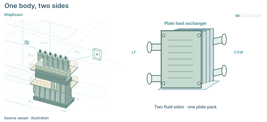
Three-dimensional arrangement explains shape and spatial relationships. A cutaway retains the machinery space’s position within the vessel. The cooler detail shows LT and CSW connections on separate fluid sides of one plate pack: heat crosses the plates while the fluids remain separate. This connects form with function.
Geometry alone cannot establish pressure, flow or temperature. A physical calculation also needs connectivity, component characteristics, commands, initial conditions and boundary conditions. The current presentation has source identity and geometry, but no actual operating records. Its later cooling example must therefore be read separately from the installed vessel system. A convincing spatial representation does not, by itself, validate physical performance.
Select the image to open it at full size.
Building the component-level explanation
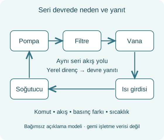
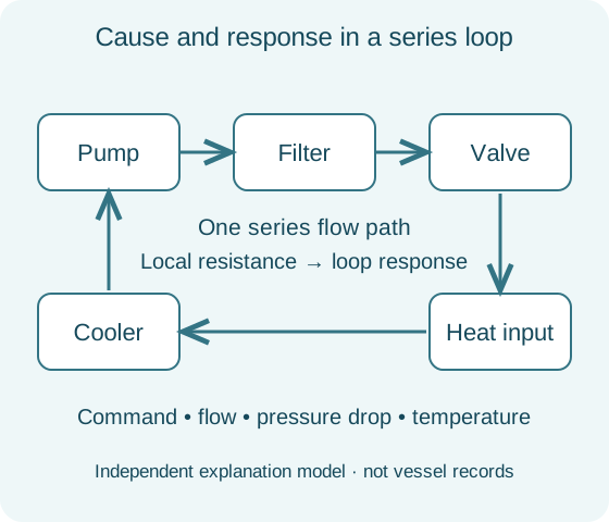
The example connects a pump, filter, valve, heat input and cooler in a series water circuit. The pump drives circulation; the filter and valve resist it. Heat enters at one component and leaves at the cooler. The initial reference uses a 300 kW heat input and 18 m³/h flow. That example flow and the source pump’s 82 m³/h rating belong to different contexts.
The cooler rejects heat toward a fixed 25 °C boundary; no separate seawater circuit is solved. Returning water retains the effect of earlier heating, so a new command does not reset temperature instantly. A differential-pressure sensor samples both sides of the filter without becoming another component in the series water path.
Learning the normal response patterns
Before introducing restriction, the example changes one input at a time. Reducing the pump command with valve and heat unchanged lowers both flow and clean-filter pressure loss. Low flow alone therefore does not prove a restricted filter. Restoring the command recovers flow, while temperature still reflects the earlier period of reduced circulation.
Next, the valve is throttled with the pump fixed. Local loss increases at the valve, while flow and clean-filter loss fall. Finally, heat input rises to 420 kW without changing pump or valve commands. Temperature responds while flow stays unchanged. These contrasting patterns establish a reference for identifying which input changed and where its effect first appears.
Testing the restriction under matched conditions
Filter resistance then increases with pump and valve commands unchanged. Flow falls, but pressure loss across the filter grows. Unlike the earlier tests, the added loss is located at the filter. Because all water in this series circuit passes through it, the local restriction affects circulation throughout the loop. The hot outlet subsequently warms as less water carries the same heat input.
The comparison uses two model cases at 810 seconds, 420 kW and identical commands. Clean-case flow is 18 m³/h, versus approximately 13.61 m³/h with restriction. Filter loss increases from about 19.62 to 179.38 kPa; the restricted hot outlet is 5.62 °C warmer. These are illustrative model results under matched conditions, not vessel measurements.
Intervention is separate from recovery
The intervention sequence separates actions that can otherwise look equivalent. Reducing heat does not remove filter resistance. Removing heat input does not instantly remove stored thermal energy. Stopping the pump takes flow to zero but does not clear the restriction. Restoring the filter, removing isolation and restarting the pump are distinct model actions; an open path alone does not create circulation.
The load then returns to 300 kW for comparison with the initial reference. Flow and filter loss recover before temperatures settle. Final temperatures are close to their starting values, not identical. This is an explanatory scenario, not a vessel maintenance procedure. Its lesson is to distinguish completing an intervention from recovering every relevant physical state.
Reading outputs: state, signal and time
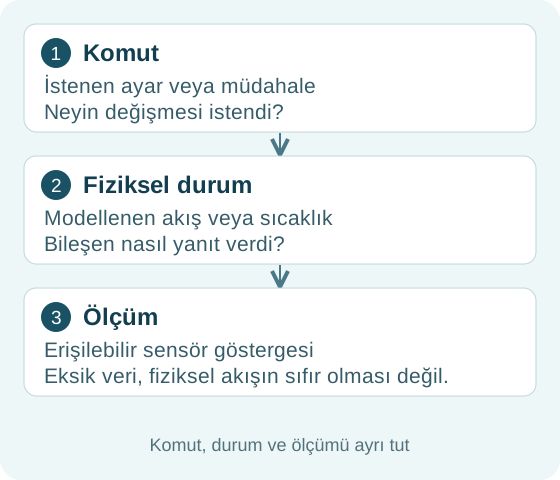
The outputs are linked records of commands, flow, pressure differences and temperatures, followed by matched comparisons. Model time differs from animation playback time, and inspecting a historical record does not move the physical process back to that instant. Record time, load and commands must be read together.
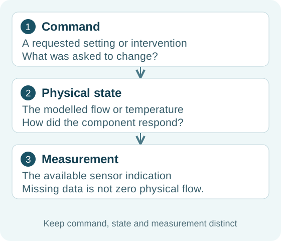
Between model seconds 1090 and 1150, the pressure-difference signal becomes unavailable while the physical process continues. The missing value is not displayed as zero pressure or stopped flow. Nor is the model’s physical value represented as a sensor reading during the gap. Calculated state, reported measurement and information availability remain three separate questions.
Current scope and the path beyond it
The current presentation pairs source-informed vessel geometry with independent cooling records. It does not demonstrate a validated whole-ship simulation, a live operational twin, automatic diagnosis, automatic repair or certification. Its contribution is to make relationships understandable while keeping the evidence behind each claim visible.
Extending this approach to operational decisions on a particular vessel would require verified installed connectivity, appropriate component characteristics and comparisons against reliable, time-aligned measurements. Sensor validity, uncertainty and deviations across operating conditions would also need assessment. These are development and validation requirements, rather than completed features of this demonstration. The foundation shown here is a disciplined workflow: locate the component, establish the conditions, follow the response and interpret the result with its evidence.